Most discussions of filters focus on their frequency response functions, which indicate the effects of the filter in the frequency domain. But do you actually care about the frequency content of your ERP waveforms? Probably not. If you’re interested in conventional ERP waveforms (as opposed to time-frequency analyses), then you probably want to know how filters change your data in the time domain, not in the frequency domain.
Filters can be implemented either in the frequency domain (using the Fourier transform) or in the time domain (using convolutions). These two approaches yield exactly the same results, but I find that the time domain implementation makes it easier to understand exactly how a filter changes an ERP waveform. So, we’ll mainly focus on the time domain for the remainder of this chapter. We’ll start with an exercise designed to help you understand time-domain filtering visually, without any math. There are many types of filters, and I’m going to focus on a common class called finite impulse response filters, even though this ends up being a slight oversimplification for the filters implemented in ERPLAB.
The key to understanding filtering in the time domain is to understand something called the impulse response function. A filter’s impulse response function is simply the output of the filter when the input is an impulse of amplitude 1 at time zero. (An impulse is a waveform that is zero everywhere except for a nonzero value at a single time point). To see what I mean, quit and restart EEGLAB, load the ERPset file named impulse0.erp, and plot the ERP waveform. When you plot this example (and the remaining examples in this chapter), make sure you set Baseline Correction to None in the GUI for plotting ERP waveforms (see the box below if you want to know why this is necessary).
Baseline Correction
The waveform in impulse0.erp has a value of 1 at time zero and a value of 0 everywhere else. The value of 1 at time zero messes up the baseline when you try to plot the waveform. This is because the baseline is defined as the average of the period up to and including time zero. This average is slightly greater than zero, and baseline correction involves subtracting the average from every point in the waveform. Thus, the whole waveform ends up being shifted slightly downward
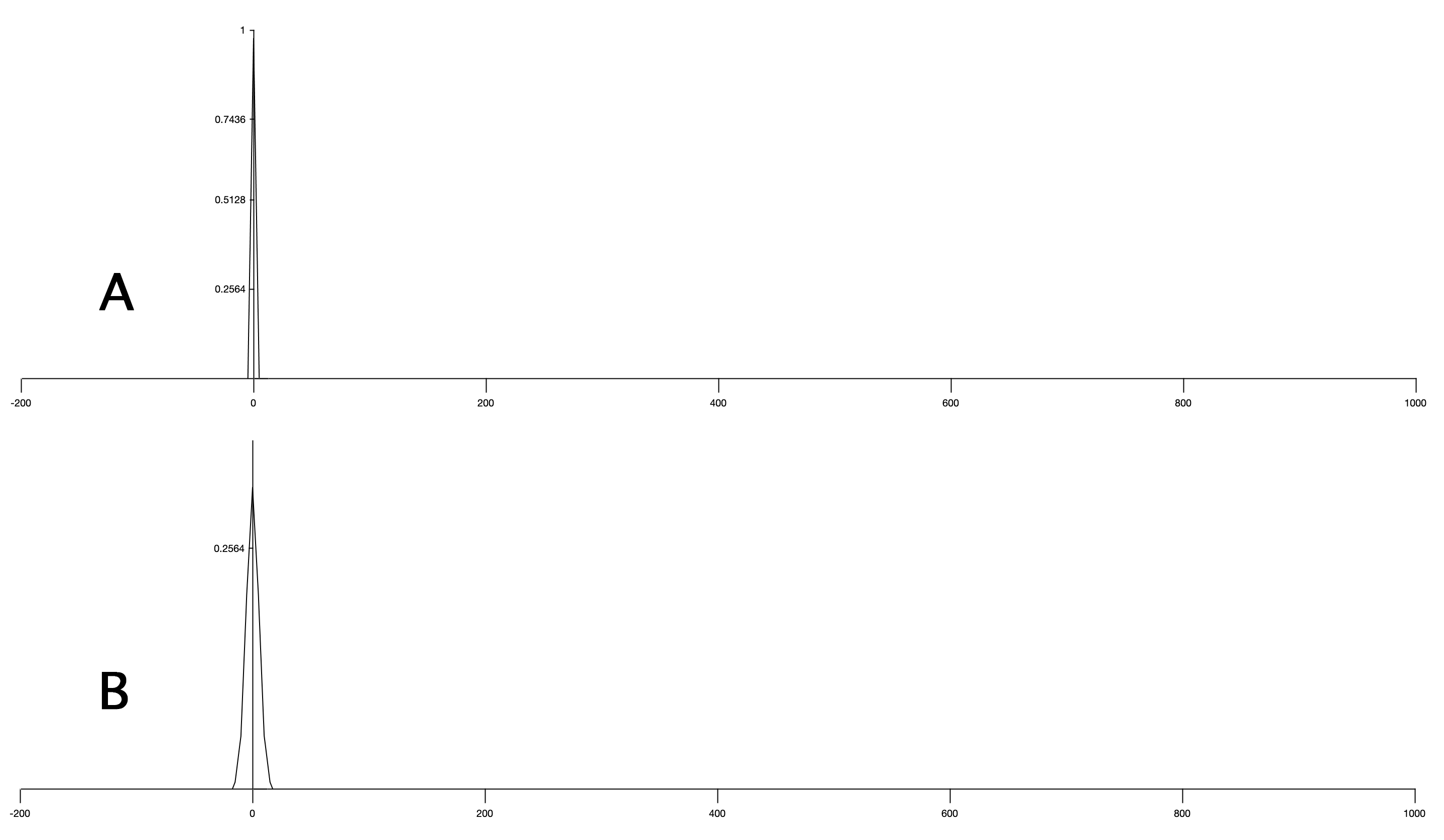
Once you’ve turned off the baseline correction, you should see something like Screenshot 4.7.A when you plot the ERPset.
Screenshot 4.7
This ERPset contains a single channel in a single bin, and you can see the impulse (a voltage of 1 µV) at time zero. It looks like a narrow triangle rather than a pure impulse because the waveform is sampled at 200 Hz (one sample every 5 ms), so there is a line going from 0 µV at -5 ms to 1 µV at 0 ms and back down to 0 µV at 5 ms.
Now filter this waveform using a half-amplitude cutoff at 30 Hz and a slope of 12 dB/octave (following the same steps you used in the previous exercise) and plot the result (which should look like Screenshot 4.7.B). You can see that the filtered waveform is now a little wider and peaks at a lower amplitude (approximately 0.32 µV). This filtered waveform is the impulse response function of the filter (i.e., the waveform produced by filtering an impulse of amplitude 1 at time zero).
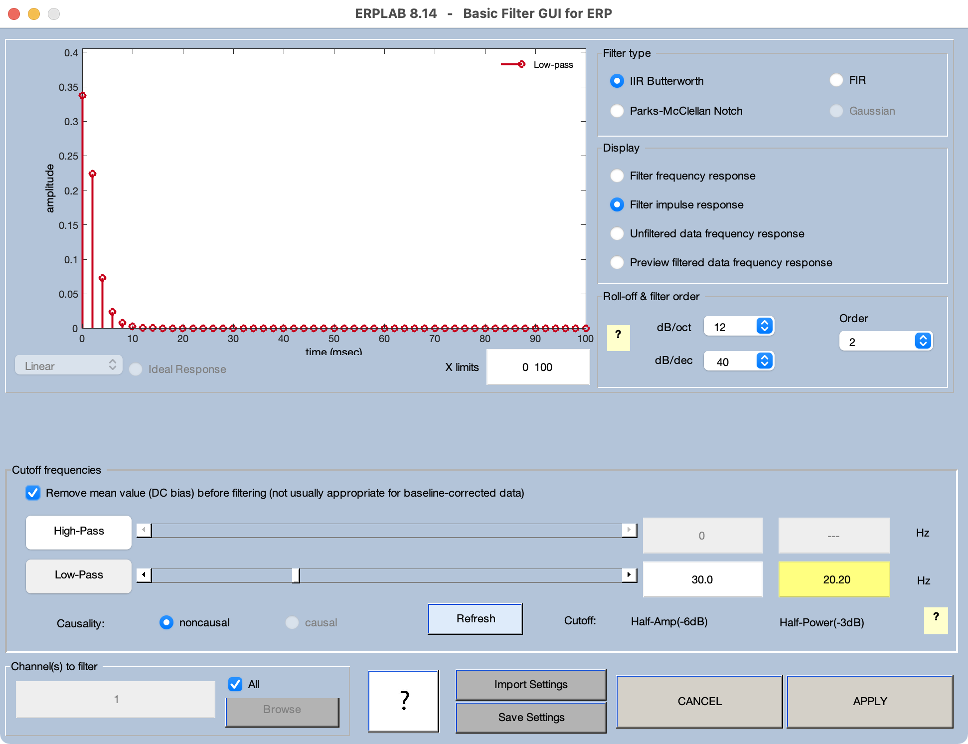
You don’t actually need to filter an impulse to see the impulse response function in ERPLAB. You can also see it by going to the window for the filtering routine and changing Display from Filter frequency response to Filter impulse response. As you can see from Screenshot 4.8, the impulse response function is now plotted. Only the right half of the function is shown, but the left half is just the mirror image. Note that it peaks at approximately 0.32 µV, just like the waveform you created by filtering an impulse (Screenshot 4.7.B). The time scale is expanded, so it’s easier to see the details of the waveform.
Screenshot 4.8
At this point, you’re probably wondering, “Why should I care what the output of a filter looks like when the input is an impulse? That impulse doesn’t look much like an ERP waveform.” You should care because the key to understanding filtering is that an ERP waveform is a sequence of voltages, one at each time point, and you can think of this as a sequence of impulses of different amplitudes. By knowing what the filter’s output looks like for an impulse at one time point (i.e., the impulse response function), you can know what the filter’s output will look like for the whole waveform. This is demonstrated in the next exercise.
A Slight Oversimplification
In this chapter, I discuss how finite impulse response (FIR) filters work, because they are quite easy to understand. However, ERPLAB implements filtering using a specific type of infinite impulse response (IIR) filter called a Butterworth filter. As long as you use a shallow roll-off (e.g., 12 dB/octave), ERPLAB’s filters provide a close approximation of a FIR filter. So, everything I say in this chapter is approximately correct for ERPLAB’s filters as long as you use a shallow roll-off.
The key difference between FIR and IIR filters is that the output of an IIR filter feeds back into the filter’s input. This means that the filter is nonlinear, with a response that could theoretically extend infinitely in time. The main advantage is that IIR filters require fewer coefficients than FIR filters, making them run faster and potentially reducing edge effects (which will be described later).