For finite impulse response function filters, the output of the filter for a complex waveform is simply the sum of the filter’s impulse response function for the voltages at each time point, scaled by the input amplitude at each time point. That’s a pretty complicated sentence, so in this exercise we’ll look at a couple simple examples.
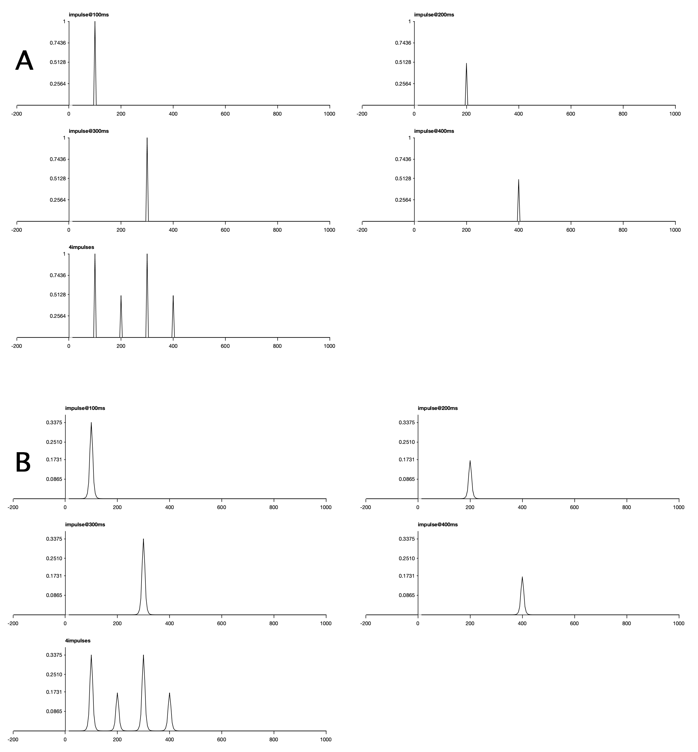
You can start by loading and plotting the ERPset file names impulse1.erp. This ERPset contains one bin, and each channel has a different impulse in it. Channel 1 has an impulse of 1 µV at 100 ms. Channels 2, 3, and 4 have impulses at 200, 300, and 400 ms with amplitudes of 0.5, 1, and 0.5 µV, respectively. Channel 5 has all four of the impulses in it (see Screenshot 4.9.A).
Screenshot 4.9
Filter this ERPset using a half-amplitude cutoff at 30 Hz and a slope of 12 dB/octave (following the same steps you used in the previous exercises) and plot the result (which should look like Screenshot 4.9.B). Each impulse has been replaced by the impulse response function of the filter, shifted so that it is centered at the latency of the impulse, and scaled (multiplied) by the size of the impulse. Importantly, filtering the waveform with four impulses (Channel 5) gives you a waveform that is equivalent to the sum of the four filtered waveforms for the individual impulses (Channels 1-4). This shows you what I meant when I said that “the output of the filter for a complex waveform is simply the sum of the filter’s impulse response function for the voltages at each time point, scaled by the input amplitude at each time point.” That is, the output of the filter for the waveform with four impulses (Channel 5) is equivalent to replacing each individual impulse with a copy of the impulse response function that has been shifted to be centered on a given impulse and scaled by the amplitude of that impulse.
To make this even clearer, we’re going to take the four impulses and make them consecutive sample points (just as an ERP waveform typically consists of a sequence of consecutive nonzero voltage values). Load the ERPset named impulse2.erp and plot it. You’ll see that now our four impulses are at 100, 105, 110, and 115 ms, which are consecutive because we have a sampling rate of 200 Hz and therefore a voltage value every 5 ms. Filter this ERPset using a half-amplitude cutoff at 30 Hz and a slope of 12 dB/octave (just as before) and plot the result. Just as in the previous example, filtering the set of four consecutive impulses is equivalent to filtering each impulse separately and then summing them together. In other words, the filtered waveform is equivalent to replacing each impulse in the unfiltered waveform with a copy of the impulse response function, centered on each impulse and scaled by the height of each impulse.
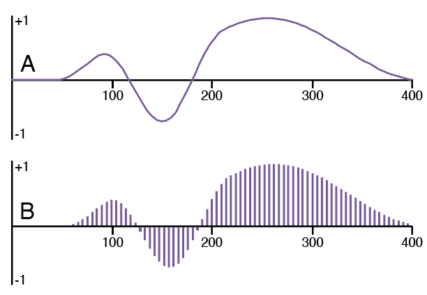
In this exercise, we used impulses to create 4 time points in an ERP waveform. Figure 4.1 extends this idea to a more realistic ERP waveform. Panel A is the same artificial waveform shown at the beginning of the chapter in Screenshot 4.1, but blown up. We have a voltage value every 5 ms, and these voltage values are connected by lines to create a waveform. Panel B is the same set of voltage values, but with the voltage at each time point shown as an impulse. This is conceptually identical to the set of four impulses shown in Screenshot 4.9.A, except now we have an impulse at each time point. To filter this waveform, we just replace each of these impulses with a copy of the impulse response function, centered at each impulse and scaled (multiplied) by the amplitude of the impulse. We then sum together these scaled copies of the impulse response function to obtain our filtered ERP waveform.
The process of replacing each point in one waveform with a scaled copy of another waveform is called convolving the two waveforms. So, filtering an ERP waveform is achieved by convolving the waveform with the impulse response function. It turns out that convolution is not as complicated (or convoluted) as it sounds!
Figure 4.1. Two ways of drawing the same ERP waveform. The waveform consists of a sequence of discrete voltage values, one at each sample point (every 5 ms in this example). We typically connect these points with lines to make it look like a continuous waveform (A). However, we can also think of each sample point as an impulse going from zero to the voltage value at that point (B). We can then think of filtering as replacing each of these impulses with a copy of the impulse response function, scaled (multiplied) by the amplitude of the impulse.
I hope you can now see that filtering in the time domain is conceptually very simple as long as you know the impulse response function of the filter. That’s why we designed the filtering tool in ERPLAB to show you this function. Many EEG/ERP analysis systems don’t show you the impulse response function, but you can always figure it out by making a waveform that consists of a single impulse (like the one shown in Screenshot 4.7.A) and passing it through the filter.
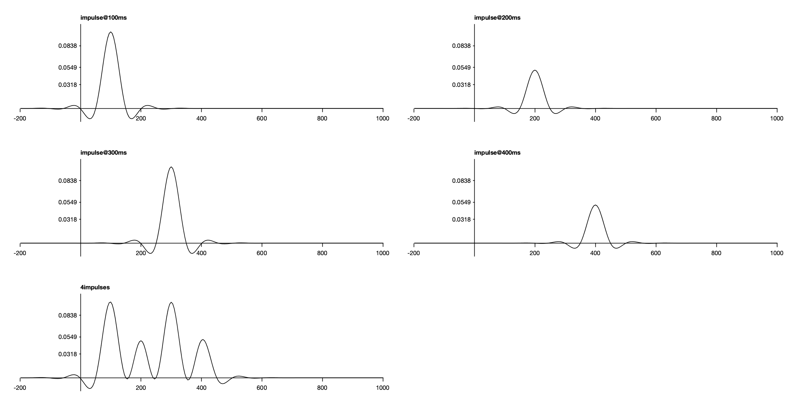
By knowing the impulse response function, you can make a pretty good guess about how the filter might distort your data. For example, do you remember the artificial negative peak produced by the filter with the 10 Hz cutoff and 48 dB/octave roll-off (Screenshot 4.6)? That artificial peak makes perfect sense once you see the impulse response function of the filter. To see the impulse response function for this filter, load the impulse1.erp ERPset (or make it the active ERPset if it’s already loaded) and filter it using a 10 Hz half-amplitude cutoff and a roll-off of 48 dB/octave. If you plot the filtered data, you’ll see something like Screenshot 4.10.
Screenshot 4.10
Channel 1 shows you what the impulse response function looks like (but centered at 100 ms rather than 0 ms because the impulse was at 100 ms). It has a negative dip on each side of the peak. And when we filter the set of four impulses in Channel 5, we can see this dip just before the first positive peak. Now imagine what happens when you apply this filter to the more realistic waveform shown in Figure 4.1.A. This would involve replacing each point in the waveform with a scaled copy of the impulse response function. When we replace the positive impulses that start around 50 ms with this function, the negative part of the impulse response function generates the negative dip prior to 50 ms.
This sort of distortion is easy to understand when you think about filtering in the time domain using the impulse response function. However, the distortion is not at all obvious when you think about filtering using the frequency response function. That’s why I prefer to think about filtering in the time domain. However, it’s still useful to know the frequency response function, especially if you know something about the frequency content of the noise in your data. This is why we designed the ERPLAB filtering tool to provide you with both functions. Also, the frequency response function and impulse response function are very closely related: The frequency response function is simply the Fourier transform of the impulse response function, and the impulse response function is simply the inverse Fourier transform of the frequency response function.