I hope it’s now clear that filtering works by replacing each point in the waveform with a scaled copy of the impulse response function. However, it’s probably not obvious why this ends up filtering out the high frequencies. There’s a slightly different—but mathematically equivalent—way of thinking about filtering that makes it more obvious.
Let’s start by forgetting everything you know about EEG and filtering, and instead think about stock market prices. Figure 4.2.A shows the daily values of the Standard & Poor 500 Stock Index over a 3-month period. There are lots of day-to-day variations that are largely random and don’t mean much for the overall economy. What would be an easy way to minimize these day-to-day fluctuations so that you could better visualize the overall trend?
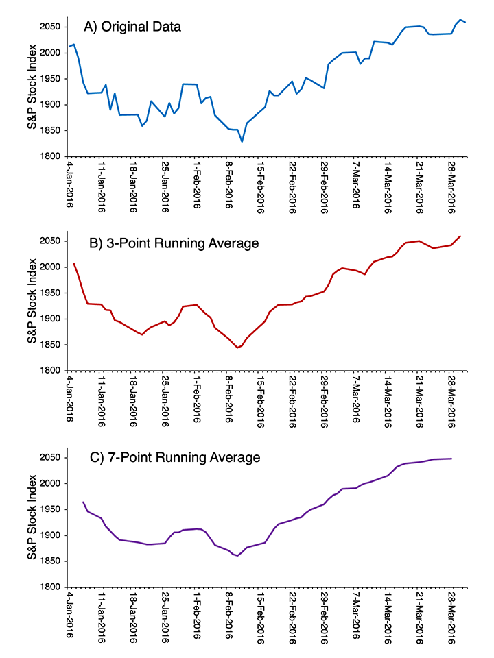
Figure 4.2. A) Standard & Poor 500 Stock Index daily values between January 4 and March 31 of 2016. B) Values after applying a 3-point running average. C) Values after applying a 7-point running average.
A common approach is to take a running average. Figure 4.2.B shows a 3-point running average of the values in Figure 4.2.A. Each value for a given day in the running average is just the average of the values from the day before, that day, and the day after. For example, the running average value on February 2 is the average of the values on February 1, 2, and 3. You can see that the running average is smoother than the original data.
We can make the data even smoother with a 7-day running average (Figure 4.2.C). Now, the running average for a given day is the average of the value on that day, the three days before, and the three days after. The more points we include in our running average, the more we attenuate rapid day-to-day changes and see the slower trends in the data. In other words, increasing the number of points in the running average increases the filtering of high frequencies in the data. So, taking a running average is a simple form of low-pass filtering, and we can control the cutoff frequency by changing the number of points being averaged together. We can apply this same algorithm to filter out high frequencies in the EEG or in ERPs (see Chapter 7 in Luck, 2014 for additional details).
Edge Artifacts
The running average approach to filtering exposes a problem that we always face in filtering, no matter what algorithm we use. The S&P 500 index values shown in Figure 4.2.A start on January 4 and end on March 31. To compute the 3-point running average value for January 4, we would need values for January 3, 4, and 5, but we don’t have the value for January 3. Similarly, we can’t calculate the running average value for March 31 because we don’t have the value for April 1. Things are even worse for the 7-point running average because now we need 3 days before and 3 days after a given day. As a result, we can’t calculate the running average for January 4, 5, or 6 or for March 29, 30, or 31 with the data that are available to us. You can see that these points are missing from the running averages in Figure 4.2.
This problem is less obvious when we filter using impulse response functions or the Fourier transform, but the same problem is present for all filtering algorithms. We solve this problem in ERPLAB using an extrapolation algorithm to estimate the values for the points that are needed but unavailable. It works quite well in most cases, but it can lead to problems when too many points must be extrapolated. The most common situation where that arises is when we use a high-pass filter to filter out low frequencies from the continuous EEG, which requires a very large number of points before and after the current point. In this situation, we sometimes see “edge artifacts” at the beginning and end of the EEG waveforms. To avoid these edge artifacts, I recommend recording an extra ~10 seconds of data prior to the first stimulus at the beginning of each trial bock and another ~10 seconds after the last stimulus at the end of each trial block. That way, the edges of the waveforms are far from the period of time you care about, and the edge artifacts occur during a time period that is outside the epochs that you will use for averaging.
In addition, ERPLAB's filtering tool has an option that can help reduce edge artifacts. This option is labeled "Remove mean value (DC offset) before filtering". It should ordinarily be used when you are filtering continuous EEG data. However, it should not be used for baseline-corrected data (e.g., epoched EEG or averaged ERPs) because the baseline correction already eliminates the DC offset (and typically works better than removing the mean value).