The advantage of the running average approach to filtering is that it’s really easy to see why it reduces high-frequency fluctuations: Any little “uppies and downies” within the set of points being averaged together will cancel each other out. Imagine that we applied a running average filter to raw EEG, using a running average width of 50 ms (e.g., 5 points on either side of the current point if we have one point every 5 ms). If the EEG has a 20 Hz sine wave in it, there will be exactly one cycle of the sine wave in 50 ms, and the positive and negative sides of the sine wave will cancel each other out.
The disadvantage of the running average filter is that it’s a bit crude. Imagine that we had a 101-point running average filter (the number is always odd because we have the current point plus an equal number of points on either side). The filtered value at time point t would be just as influenced by time point t-50 as by point t-1. Instead of giving all 101 points equal weight, it would make more sense to give nearby points greater weight than more distant points. That’s actually quite easy to do.
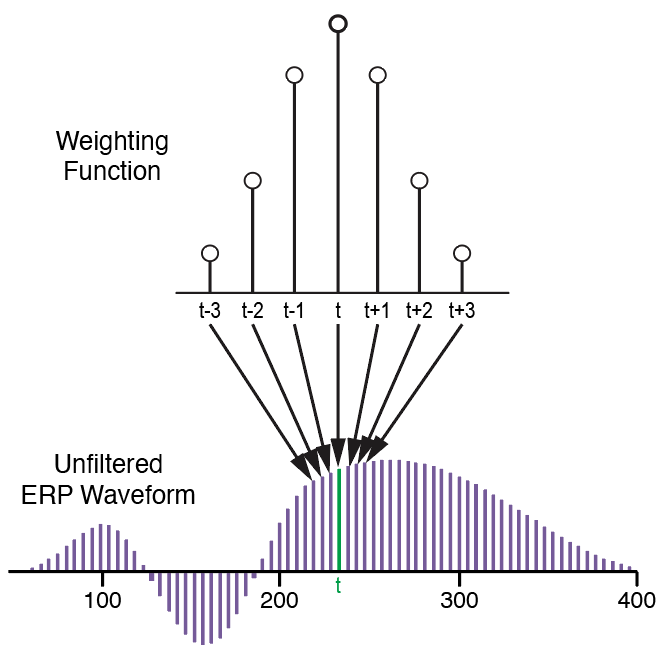
This weighted running average approach to filtering is illustrated in Figure 4.3. We start by defining a weighting function, which indicates how much weight each of the surrounding time points will have. For example, rather than having a 7-point running average in which each of the 7 points has equal weight, the 7-point weighting function shown in Figure 4.3 gives the greatest weight to the current point, and then the weights fall off for more distant points. The filtered value at time t is computed by taking each of the 7 points (t-3 through t+3), multiplying the unfiltered value at each point by the corresponding value from the weighting function, and the summing these weighted values.
Figure 4.3. Filtering with a weighting function. To calculate the filtered value at time t, you take each of the surround points (t-3 through t+3), multiply the unfiltered value at each point by the corresponding value from the weighting function, and sum them together.
A standard 7-point running average could be computed in the same way. Our weighting function would have a value of 1/7 at each of the 7 points. The filtered value at time t would then be computed by taking 1/7 times the voltage at each of the 7 points and then summing these values together. That’s identical to taking the average of the 7 points.
I hope that you can still see how this more sophisticated version of the running average filter will tend to attenuate high frequencies: Uppies and downies during the set of points being averaged together will tend to cancel each other out.
You may be wondering how this weighted running average approach is related to filtering with an impulse response function. The answer is beautifully simple: The weighting function is simply the mirror image of the impulse response function. And if the impulse response function is symmetrical (which is usually the case), the weighting function is exactly the same as the impulse response function. Also, because the weighting function is just the mirror image of the impulse response function, you can compute the frequency response function by applying the Fourier transform to the mirror image of the weighting function.
The only real difference between filtering with an impulse response function and filtering with a weighting function is conceptual: the impulse response approach tells you how the unfiltered value at time t will influence the filtered values at the surrounding time points (because the unfiltered value at time t is replaced by a scaled copy of the impulse response function), whereas the weighted running average approach tells you how the filtered value at time t is influenced by the unfiltered values at the surround points (because the filtered value at time t is the weighted sum of the surrounding time points).
Thinking about filtering in terms of the weighting function should help you understand an important consequence of filtering: Filtering inevitably reduces temporal resolution (no matter how the filtering is implemented). The filtered value at a given time point is influenced by the surrounding time points, so the voltage you see at 100 ms is now influenced by the voltages at 95 ms, 105 ms, etc. And the weighting function shows you exactly how much impact the preceding and subsequent time points will have on the filtered value at a given time point. The wider the weighting function, the more you are filtering your data, and the more temporal precision you have lost. This is a very clear example of the principle that increasing the precision in the frequency domain (by limiting the set of frequencies that are in the filter output) decreases the precision in the time domain (by causing the filtered value at a given time point to be influenced by a wider range of time points from the unfiltered data).