Now let’s take a closer at how low-pass filters reduce temporal resolution. The general idea is that each point in the unfiltered waveform gets replaced by a scaled copy of the impulse response function, so the filtered data get “spread out” by the width of the impulse response function. Let’s look at an example.
Load the ERPset named peak1.erp and plot it. You’ll see that there are three identical channels, each with a single peak at 100 ms. We’re going to leave Channel 1 unchanged and we’re going to filter Channels 2 and 3 with different filter cutoffs. To do this, launch the filtering tool (EEGLAB > ERPLAB > Filter & Frequency Tools > Filters for ERP data) and set it to filter the data with a low-pass cutoff at 30 Hz and a roll-off of 12 dB/octave. Then, in the lower left corner of the window, change Channel(s) to filter to be 2 instead of having the All box checked. This will apply the filter only to Channel 2. Click APPLY and then specify whatever ERPset name you’d like. Now launch the filtering tool again, and change the cutoff to 10 Hz (leaving the roll-off at 12 dB/octave). Change Channel(s) to filter to be 3 instead of 2, click APPLY, and use whatever ERPset name you’d like.
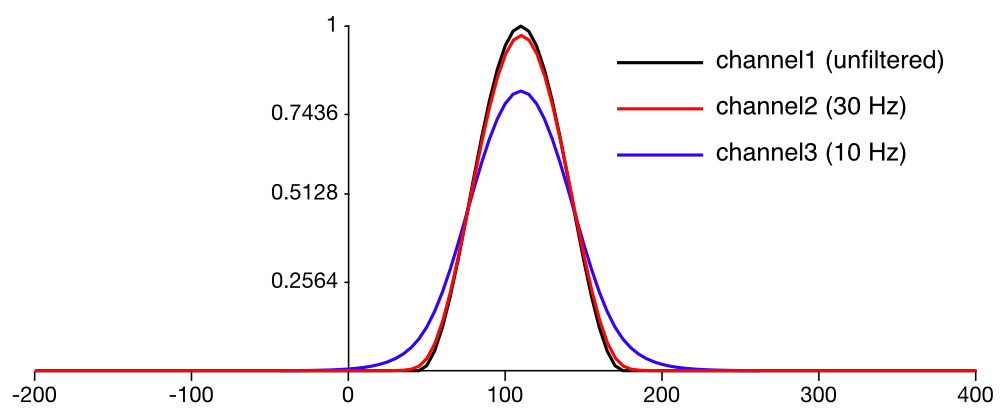
Plot the ERPs to see the effects of the filtering. Channel 1 has not been changed. Channel 2 has been filtered at 30 Hz, but it will look only slightly different from Channel 1 because this is a pretty minimal filter. Channel 3 has been filtered at 10 Hz, and if you look closely, you’ll see that the waveform in Channel 3 onsets significantly earlier and offsets significantly later than the original waveform in Channel 1.
To make it easier to compare the waveforms, I overlaid them in Figure 4.4. You can see that the 30-Hz filter had almost no effect, but the 10-Hz filter caused the waveform to “spread out,” making the onset earlier and the offset later. It also decreased the peak amplitude (because the original waveform had significant power in the frequencies around 10 Hz that has now been eliminated).
Now let’s see how these effects can be explained by the impulse response function of the filter. Go back to the filtering tool, and check the All box for Channel(s) to filter. Leave the cutoff frequency at 10 Hz and change the Display setting near the top from Filter frequency response to Filter impulse response. Remember, only the right half of the impulse response function is shown; the left half is the mirror image of the right half. You can see that the impulse response function extends for about 30 ms. This means that any activity in the unfiltered waveform will be spread approximately 30 ms both leftward and rightward.
A Frustrating Moment
I forgot to set Channel(s) to filter back to All the first time I ran through this exercise. The next time I filtered an ERP, it seemed like the filtering wasn’t working because only one channel was being filtered. I tried restarting ERPLAB, and that didn’t help. I tried restarting Matlab, and that didn’t help either. I was getting frustrated and was about to reset ERPLAB’s working memory (which would have helped, because it would have reset all the filtering options to their defaults), but then I noticed that the All box wasn’t checked. I checked it, and then everything started working as expected. This is just one of many times that I ran into a problem while creating the exercises in this book and used the troubleshooting steps described in Appendix 1. The moral of the story is that even the guy who oversaw the design of ERPLAB and has decades of experience with analyzing ERPs runs into problems from time to time!
Now change the half-amplitude cutoff from 10 Hz to 30 Hz and look at the impulse response function. It now declines to near zero within 10 ms. This means that the spreading produced by this filter will be less than ~10 ms. Note that the visual appearance of the spreading will depend on the shape of the waveform. For example, the spreading in Figure 4.4 looks more than 3 times greater for the 10 Hz filter than for the 30 Hz filter. However, you could see that this what is happening if you filtered an impulse. You could also see the 10-ms spreading for the 30 Hz filter if you zoomed in sufficiently closely.
Figure 4.4. Artificial waveform without filtering, with a 30-Hz half-amplitude cutoff, and with a 10-Hz half-amplitude cutoff.