Up to this point, we’ve focused on low-pass filters, but in this exercise we’ll see how high-pass filtering works. The only fundamental difference is that the impulse response functions are different.
With typical parameters (e.g., a 0.1 Hz half-amplitude cutoff frequency), high-pass filtering requires a very long impulse response function, so it doesn’t work very well with epoched EEG or ERP data (unless the epochs are many seconds long). Ordinarily, you’ll apply high-pass filtering to continuous EEG (as in some of the exercises in earlier chapters). However, it’s a little easier to create simulated waveforms and visualize them with ERPs, so we’ll apply high-pass filters to simulated ERP data in this exercise. As a compromise, I created simulated waveforms with a longer-than-usual epoch (from -1000 to +1000 ms). But with real data, you’d want even longer epochs (or, better yet, apply high-pass filters to the continuous EEG data).
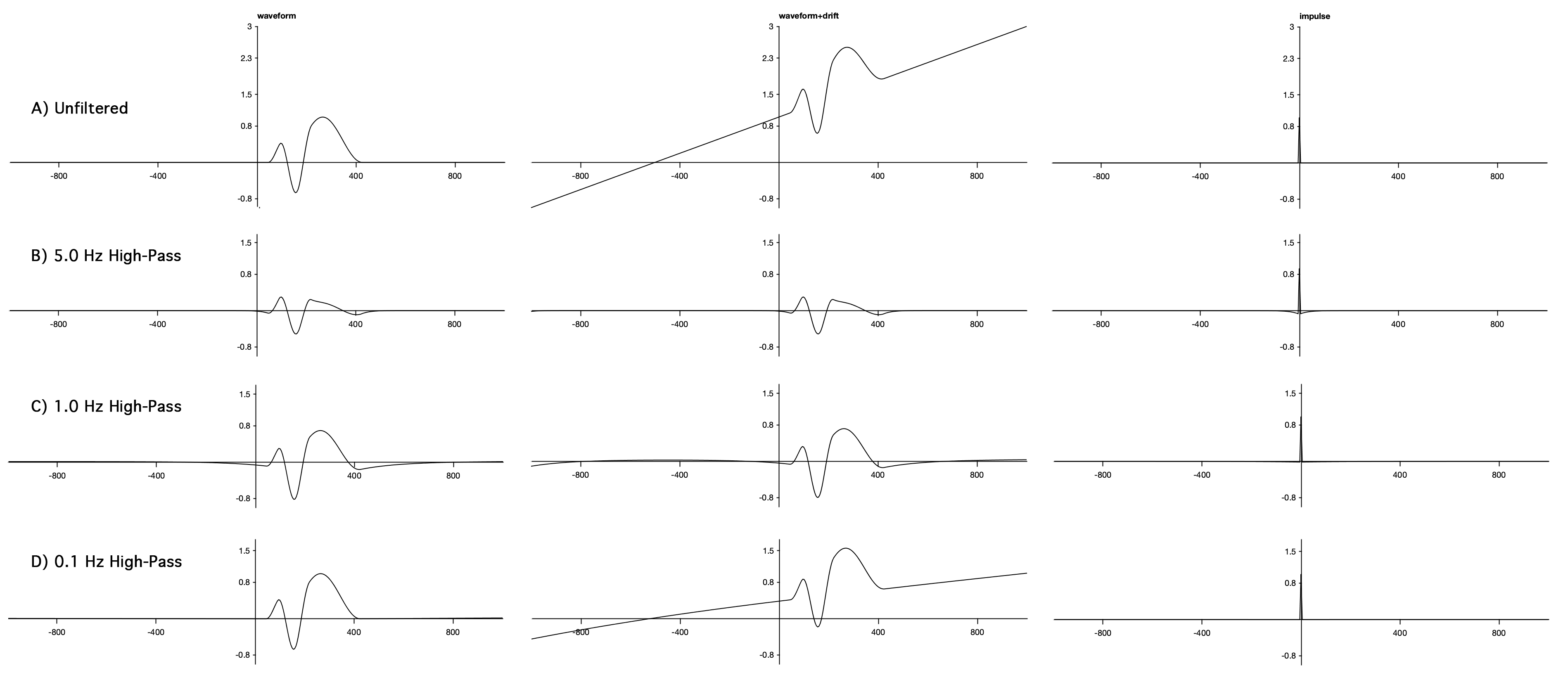
To get started, quit and restart EEGLAB and then load the ERPset in the file named waveform+drift.erp. If you plot the ERPs, you’ll see something like Screenshot 4.11A. Channel 1 is the same artificial waveform we’ve used before, but with a longer epoch. Channel 2 is the same waveform, but with a linear drift superimposed on it. Channel 3 is an impulse that we can use to visualize the impulse response functions of the filters we’ll be using.
Screenshot 4.11
We’re going to start by using a high-pass filter cutoff of 5 Hz, which means that we’re filtering out frequencies below 5 Hz. I’d never recommend using this cutoff with real data (except for a few special cases, such as research on the auditory brainstem response). However, this will make it easier to see what the impulse response function looks like and how it impacts the filtered waveform.
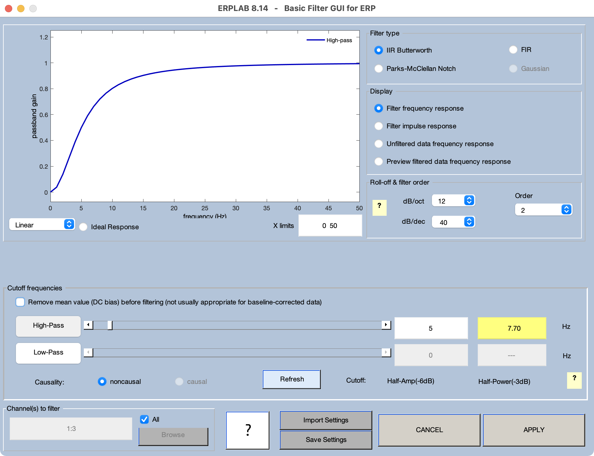
Launch the filtering tool, and set the parameters as shown in Screenshot 4.12. In particular, turn off the low-pass filter, turn on the high-pass filter, set the high-pass cutoff to 5 Hz, and set the roll-off to 12 dB/octave. And make sure that Channel(s) to filter is set to All. If you look at the frequency response function shown in the upper left, you’ll see that the gain is near zero for the lowest frequencies, reaches 0.5 at 5 Hz (because that’s the half-amplitude cutoff frequency) and then starts nearing the asymptote of 1.0 by approximately 10 Hz.
Screenshot 4.12
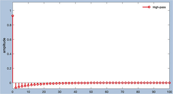
Now look at the impulse response function by changing the Display setting from Filter frequency response to Filter impulse response. It should look like Screenshot 4.13. It’s very different from the impulse response function of a low-pass filter. Low-pass and high-pass filters have opposite effects (removing high versus low frequencies), so they have largely opposite impulse response functions. Whereas the low-pass impulse response functions we’ve looked at had positive values near time zero, this high-pass impulse response function is negative near time zero (but is near 1.0 right at time zero). The reasons for this are discussed in Chapters 7 and 12 of Luck (2014). Here, you’ll just have to take my word for it.
Screenshot 4.13
Go ahead and click APPLY to run the filter, and then plot the filtered waveforms. You should see something like Screenshot 4.11B. First look at the impulse (Channel 3), which now shows the impulse response function of the filter. You can see the negative values surrounding time zero, but they’re pretty small. This is because the impulse response function for a high-pass filter must sum to zero. If the impulse response extends for a long time period, the individual values must be very small.
Now look at the waveform+drift channel (Channel 2). The good news is that the filter has virtually eliminated the drift. The bad news is that the filter has produced artifactual negative peaks at the beginning and end of the waveform. You can also see these artifactual peaks in the channel without the drift (Channel 1). The filter has also reduced the amplitude and change the shape of the ERP waveform, but that’s to be expected because much of the power in the waveform falls into the frequencies that are attenuated by the filter (which you can confirm by making the unfiltered ERPset active and using EEGLAB > ERPLAB > Filter & Frequency Tools > Plot amplitude spectrum for ERP data). These distortions are why I would never recommend using a filter like this with real data (except for the auditory brainstem responses, which are largely confined to higher frequencies).
If you think about the impulse response function, you can understand why the filter produces artificial negative peaks at the beginning and end of the waveform. The unfiltered waveform starts and ends with positive values. When we replace these values with the impulse response function, the negative values to the left and right of the current point in the impulse response function produce negative values before and after the positive peaks. Note that if the waveform contained negative peaks, the artifactual peaks would be positive (because a negative voltage from the unfiltered waveform multiplied by a negative value in the impulse response function creates a positive value).
Next we’re going to try a filter that’s not quite as extreme, but still has a higher cutoff frequency than I’d recommend, namely 1 Hz. Make the original waveform+drift ERPset active again in the ERPsets menu, launch the filtering tool, and change the cutoff from 5 Hz to 1 Hz. Look at the impulse response function in the filtering tool. You can see a large positive value at time zero, but the nearby values are just barely negative. The function extends for a longer period of time than the function for the 5 Hz filter, and each individual point must be nearer to zero so that the points sum to zero.
Go ahead and click APPLY and then plot the filtered data. It should look like Screenshot 4.11C. The drift in Channel 2 is still largely gone, but we haven’t attenuated the ERP waveform as much, so that’s an improvement. However, the artifactual negative peaks at the beginning and end of the waveform are still present. That’s why I wouldn’t recommend using a 1 Hz cutoff.
Now let’s try the high-pass filter cutoff I ordinarily recommend for most perceptual, cognitive, and affective ERP studies, namely 0.1 Hz. Make the unfiltered ERPset active again, launch the filtering tool, and change the cutoff to 0.1 Hz. If you look at the impulse response function in the filtering tool, you can’t really see much beyond the positive value at time zero. That means that the filter will be very mild. Apply the filter and look at the waveforms. As shown in Screenshot 4.11D, the filter has only partially reduced the drift in Channel 2. However, it has produced no noticeable distortion of the ERP waveform. That is, the filter hasn’t attenuated the waveform, and it hasn’t produced any artifactual peaks.
This set of examples illustrates an important principle: You can fully attenuate the slow drifts in your data but distort your ERP waveforms, or you can fail to fully attenuate the low-frequency noise and avoid distorting your ERP waveforms. You can’t both fully attenuate the drifts and avoid distorting the waveform. This is because of the inverse relationship between the time and frequency domains: The more you restrict the frequencies with extensive filtering, the more you distort the time course of the ERP waveform.
Keep in mind that the slow drifts are noise deflections that mainly arise from the skin, and they’re positive-going on some trials and negative-going on others. They add random noise to your data, decreasing your power to find statistically significant effects. Obviously that’s not a good thing. However, it’s much worse to use a filter that induces artifactual effects that are statistically significant but completely bogus, causing you to draw incorrect conclusions. This is why I usually recommend a high-pass cutoff of 0.1 Hz—it reduces the low-frequency noise reasonably well, but it doesn’t usually produce substantial artifacts.
In the first edition of my ERP textbook (Luck, 2005), I recommended using 0.01 Hz as the half-amplitude cutoff. Over the following years, however, my collaborators and I systematically compared a variety of different cutoffs, and we typically found that 0.1 Hz produced the best noise reduction without any substantial distortion of the waveforms (Kappenman & Luck, 2010; Tanner et al., 2015). If you’re looking at very slow ERPs (like the contralateral delay activity), 0.01 or 0.05 might be better than 0.1, but in most cases I find that 0.1 Hz works best.