In this exercise, we’re going to create response-locked averages rather than stimulus-locked averages. That is, when we create our EEG epochs, the event code for the response will be time zero.
An important feature of BINLISTER is that it does not make a distinction between stimulus events and response events. An event code is an event code, no matter whether it represents a stimulus, a response, an eye movement, a heartbeat, or a sudden change in the FTSE stock index. Any event code can be the time-locking event (time zero). And a bin can be defined by any sequence of event codes.
Open the bin descriptor file named BDF_P3_Response_Locked.txt in the Matlab text editor (by double-clicking it in the Current Folder pane). Here’s what you should see:
bin 1
Rare, Correct
{t<200-1000>11;22;33;44;55}.{201}
bin 2
Frequent, Correct
{t<200-1000>12;13;14;15;21;23;24;25;31;32;34;35;41;42;43;45;51;52;53;54}.{201}
It’s a lot like the original bin descriptor file (BDF_P3.txt). The most important change is that the period symbol in each bin descriptor is to the left of the response event list rather than being to the left of the stimulus event list. The period goes to the left of the time-locking event, so this is how we indicate that the response event code (201) will be the time-locking event. The t<200-1000> part has also been moved from the response event list to the stimulus event list. The timing is always given relative to the time-locking event, which is now the response, so we need to specify that the stimuli must be 200-1000 ms prior to the response rather that the response being 200-1000 ms after the stimulus.
If EEGLAB is running, quit it and restart it so that everything is fresh, and then load the original dataset again (12_P3_corrected_elist.set). Then run BINLISTER, using BDF_P3_Response_Locked.txt instead of BDF_P3.txt as the bin descriptor file. You can use whatever dataset names are convenient, but make sure to save the EventList as a new text file when you run BINLISTER so that you can compare it to the original version.
Take a look at the new EventList text file. If you look at the bin column on the far right, you’ll now see bin numbers on the lines for the response event codes (the 201 codes), with a 1 if the response is preceded by a target event code (11, 22, 33, 44, or 55) and a 2 if the response is preceded by a nontarget event code. This shows us that the responses will be used as time zero when we epoch and then average the data.
To see this, go ahead and epoch the data (EEGLAB > ERPLAB > Extract bin-based epochs) with the settings shown in Screenshot 6.3. Rather than using the default epoch of -200 to 800 ms, we’re now using an epoch of -600 to 400 ms. This is because much of the activity occurs before rather than after time zero in a response-locked average. Also, rather than using Pre as the baseline correction interval (which would use the period from -600 to 0 ms), select Custom and put -600 -400 into the text box as the start and stop times. This period should be prior to stimulus onset on most trials because most of the RTs are <400 ms. (There is a way to “trick” ERPLAB into using the actual prestimulus interval as the baseline in a response-locked average, but it’s too complicated for this exercise.)
Screenshot 6.3
Take a look at the epoched data (using EEGLAB > Plot > Channel data (scroll)). If you look at the first epoch, you’ll see an event code labeled B2(201) at time zero. This means that the event code was 201, and it’s now the time-locking event for Bin 2. You’ll also see that the epoch begins 600 ms before this event and ends 400 ms after the event. You can’t see the stimulus event code prior to this response, because it was more than 600 ms prior to the response and therefore falls outside the epoch. (You can verify this by looking at the diff column in the EventList text file.) However, you can see the stimulus event code prior to the response in the second epoch. The stimulus event code isn’t at time zero and it doesn’t begin with B2 because it wasn’t the time-locking event. Scroll through several pages of epochs to make sure you understand what’s in this file.
Now average the data, just as you did for the stimulus-locked data, but use 12_P3_Response_Locked when you are prompted for the name of the ERPset. Next, plot the ERPs (using EEGLAB > ERPLAB > Plot ERP > Plot ERP waveforms). In the region of the plotting GUI labeled Baseline Correction, select None. Otherwise the plotting routine will re-baseline the data using the interval from -600 to 0 as the baseline. Click PLOT to see the data.
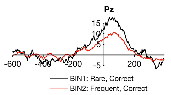
Screenshot 6.4 shows a closeup of the waveforms from the Pz channel. You can see that the brain activity now begins approximately 200 ms before the time-locking event (the response), because the stimulus is now before time zero. In addition, the P3 peaks shortly after time zero. Compare this with the stimulus-locked waveforms from the Pz site in Screenshot 6.2, where the P3 peaked around 350 ms. Given the combination of the stimulus-locked and response-locked waveforms, can you guess the approximate mean RT for this participant?
The P3b component is usually tightly time-locked to the participant’s decision about whether the current stimulus belongs to the Rare category or the Frequent category, so P3b latency usually (but not always) varies from trial to trial according to the response time As a result, it can be informative to look at the P3b waveform in both stimulus- and response-locked averages. For an example from the basic science literature, see Luck & Hillyard (1990) or the condensed description of this experiment in Luck (2014; especially Figure 8.8 and the surrounding text). For an example with a clinical population, see Luck et al. (2009).