In this exercise, we’re going to create bins for the error trials as well as for the correct trials. This will allow us to look at the error-related negativity (ERN, also called Ne), a negative-going ERP response over frontocentral electrode sites that is produced when the participant makes an obvious error (see the excellent review by Gehring et al., 2012). Errors are pretty common on the Rare trials in the oddball paradigm because the response for the Frequent category becomes highly primed. When you’re doing the task, you find yourself pressing the Frequent button even though you realize (a moment too late) that you should be pressing the Rare button.
Although the first published report of the ERN used an oddball task (Falkenstein et al., 1990), this task is less than ideal for looking at errors because error trials are a small subset of an already-rare stimulus category, leading to very few error trials. In the ERP CORE, we instead used a flankers task to look at the ERN, and we didn’t even analyze the error trials in the oddball task. In this exercise, we’re going to analyze the error trials in the oddball task and look for the ERN. Do you think we’ll see an ERN? I wasn’t sure we’d see it until I analyzed the error trials for the first time yesterday!
My first step was to create a new bin descriptor file that includes bins for the error trials. The file is named BDF_P3_Accuracy.txt—go ahead and open it in the Matlab text editor (by double-clicking it in the Current Folder pane). You’ll see that I just added bins for the Rare and Frequent stimuli followed by an error response (event code 202) instead of being followed by a correct response (event code 201).
If EEGLAB is running, quit it and restart it so that everything is fresh, and then load the original dataset again (12_P3_corrected_elist.set). Then run BINLISTER, using BDF_P3_ Accuracy.txt as the bin descriptor file. You can use whatever dataset names are convenient, but make sure to save the EventList as a new text file.
Take a look at the new EventList text file. Near the top, under the header information, you’ll see the number of trials in each bin. As before, there were 30 Rare trials followed by a correct response and 153 Frequent trials followed by a correct response in Bins 1 and 2. However, there were only 9 Rare trials followed by an incorrect response and a measly 3 Frequent trials followed by an incorrect response. And this is actually more error trials than was typical (probably because this participant’s response times were faster than those of most participants in this experiment). In the ERP CORE flankers experiment, which was designed to look at the ERN, we controlled the number of errors by telling participants to speed up if they made errors on fewer than 10% of trials and telling them to slow down if they made errors on more than 20% of trials. But the oddball experiment was not designed to look at the ERN, so we didn’t try to control the number of errors. Some participants made a lot, and some made hardly any.
As usual, the next step is to epoch the data (EEGLAB > ERPLAB > Extract bin-based epochs). The epoching routine may still have the settings from the response-locked averaging we did in the previous exercise, but now we’re going to make stimulus-locked averages, so make sure that the epoch time range is set to -200 800 and the baseline correction period is set to Pre. Click RUN and name the resulting dataset whatever you want. Now average the data. You should name the resulting ERPset 12_P3_Accuracy and save it as a file named 12_P3_Accuracy.erp. You’ll need it for a later exercise.
The averaging routine prints the best, worst, and median aSME values to the command window. You should always look at these values to make sure there isn’t a problem with the data quality. You’ll see that the maximum value is much larger than the median, which tells you there might be a problematic bin or channel. Of course, we might expect low data quality for the error trials given how few trials were present. Consistent with this, the maximum value was for the bin with Frequent stimuli followed by an incorrect response, which had only 3 trials.
Take a look at all the aSME values using EEGLAB > ERPLAB > Data Quality options > Show Data Quality measures in a table. For the correct trials (Bins 1 and 2), the values look pretty reasonable. The SME quantifies the standard error of measurement, and a standard error of between 1 and 3 µV is reasonably small relative to the >15 µV amplitude of the P3b. Now look at the values for Rare stimuli followed by an incorrect response (Bin 3). Most of the values are still less than 5 µV, which seems reasonable given the small number of trials. If you look at the values for Bin 4, however, you’ll see a lot of values that quite a bit larger. This makes sense given that we had only 3 trials in this bin.
How many trials do you need? Some researchers have tried to provide a simple answer to this question, but there is no simple answer because it depends on the number of participants (Baker et al., 2020) and the magnitude of the effect being studied (see Boudewyn et al., 2018).
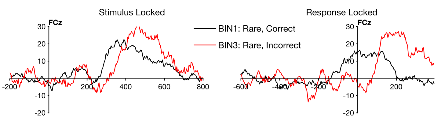
Now let’s plot the ERPs (using EEGLAB > ERPLAB > Plot ERP > Plot ERP waveforms; you may need to click the RESET button to clear out the plotting parameters we used in the previous exercise). We’ll start by plotting the correct and incorrect Rare trials, so specify Bins 1 and 3. Now we can finally answer the question of whether errors produce an ERN in this experiment (at least for this one participant). The left side of Screenshot 6.5 shows what you should see in the FCz channel, where the ERN is usually largest. You can see that the voltage is more negative from ~200-400 ms on the error trials than on the correct trials. This is the ERN! Replication is a cornerstone of science, and it sure is nice to see that this effect can be replicated.
You can see that voltage is more positive for error trials than for correct trials from ~400-600 ms. This effect has also been seen in many prior studies, and it’s called the error positivity or Pe.
Screenshot 6.5
As always, you’ll want to look at all the channels to see the scalp distribution of the effect. You can see that the difference between error trials and correct trials (both in the ERN and Pe time windows) is biggest at frontal and central midline electrode sites. This is what is typically observed when the mastoids or nearby sites are used as the reference. If you’re interested, you can try re-referencing to the average of all sites and see how this changes the scalp distribution.
You should also try plotting the correct and incorrect Frequent waveforms (Bins 2 and 4). However, it’s hard to see much because there were only 3 incorrect Frequent trials, so the waveforms are extremely noisy.
The ERN usually occurs right around the time of the response. When RTs vary greatly from trial to trial, the ERN in the stimulus-locked averages occurs at different times on different trials, and this makes the ERN look “smeared out” in stimulus-locked averages. The waveforms also look as if the P3b is just shifted to the right on the error trials. In fact, when Bill Gehring first saw the ERN, he was looking at stimulus-locked averages, and he wasn’t sure it was a real component. However, when he made response-locked averages, the ERN was a big, beautiful deflection at time zero. You can read the story of how he discovered the ERN in Chapter 3 of Luck (2014).
The participant we’ve been looking at in this chapter didn’t have a lot of RT variability, so the ERN is easily visible in the stimulus-locked averages. But let’s make response-locked averages to see if this makes the ERN even clearer. To do this, follow the instructions in the previous exercise for making a response-locked average (especially using an epoch of -600 to 400 ms), but use BDF_P3_Accuracy_Response_Locked.txt as the bin descriptor file.
For the FCz channel, the response-locked waveforms should look like those on the right side of Screenshot 6.5. Now the ERN appears as a relatively sharp negative deflection, peaking shortly after time zero (the time of the buttonpress). You can see that it’s a distinct deflection rather than simply being a rightward shift in the P3b.