A classic finding in the ERP literature is that the P3b component elicited by an oddball is smaller if the previous trial was also an oddball than if the previous trial was a standard (Squires et al., 1976). In this exercise, we will perform a sequential analysis to see this effect using the ERP CORE P3b paradigm. This will bring up some important general issues about ERPs as well as showing you more about the process of assigning events to bins.
I’ve provided a bin descriptor file for this analysis named BDF_P3_Sequential.txt—go ahead and open it in the Matlab text editor (by double-clicking it in the Current Folder pane). You’ll see that we have 4 bins: Bin 1, Rare preceded by Rare; Bin 2, Rare preceded by Frequent; Bin 3, Frequent preceded by Rare; Bin 4, Frequent preceded by Frequent. The bin descriptors were modified to require that the time-locking stimulus was preceded by either the Rare or Frequent stimulus and a correct response. For example, Bin 1 is defined as:
Okay, let’s make some ERPs with these bins. Quit and restart EEGLAB so that everything is fresh, and then load the original dataset again (12_P3_corrected.set). Now run BINLISTER, using BDF_P3_ Sequential.txt as the bin descriptor file. We’ll need the resulting dataset for a later exercise, so name it 12_P3_corrected_elist_bins_seq, and save it as a file named 12_P3_corrected_elist_bins_seq.set.
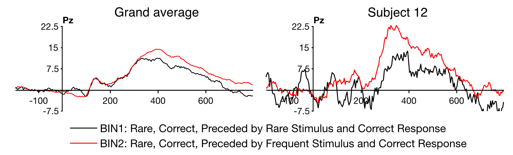
Take a look at the new EventList text file to see how many trials we have in each bin. There were only 6 Rare trials that were preceded by Rare trials (with correct responses on both trials). That’s not a lot! This was a pretty short experiment (about 10 minutes), and we would ordinarily use a longer session with a lot more trials to do a sequential analysis. In fact, when I was developing this exercise, the first subject I tried didn’t have a clear sequential effect; there was a hint of an effect, but the data were so noisy that it wasn’t very clear. I then wrote a script to do the analysis for all the participants (which is provided in the Chapter_6 folder). Fortunately, when I looked at the grand average, I saw the nice effect shown on the left of Screenshot 6.6, in which the P3b for the Rare stimulus was clearly larger when the preceding trial was the Frequent stimulus than when it was the Rare stimulus. I then looked for a participant who exhibited this effect clearly, and I used this participant (Subject 12) for all the exercises in this chapter.
Screenshot 6.6
The next step is to epoch the data (EEGLAB > ERPLAB > Extract bin-based epochs). Make sure that the epoch time range is set to -200 800 and the baseline correction period is set to Pre. Click RUN and name the resulting dataset whatever you want. Now average the data. You should name the resulting ERPset 12_P3_Sequential and save it as a file named 12_P3_Sequential.erp. Now plot the data for the Rare stimuli (Bins 1 and 2). If you look at the Pz channel, you should see something like the waveforms shown on the right of Screenshot 6.6. Once again, we’ve successfully replicated a finding from prior research!
However, we need to worry about the data quality given the small number of trials. Take a look at the aSME values for Bins 1 and 2 (EEGLAB > ERPLAB > Data Quality options > Show Data Quality measures in a table). You’ll see that most of the values are worse (higher) for Bin 1 than for Bin 2, which is not surprising given that we had 6 trials in Bin 1 and 22 trials in Bin 2. However, if you look at the Pz channel from 300 to 800 ms, you’ll see that the aSME values are only slightly higher for Bin 1 than for Bin 2. I think this was just good luck: by chance, this channel didn’t show a lot of trial-to-trial variability in P3b amplitude in Bin 1, so the standard error was pretty good despite the small number of trials. This makes the data from the Rare-preceded-by-Rare condition somewhat believable. However, the nice big effect in the grand average is what really makes it believable.
Sequence or Time?
Although many P3b effects have traditionally been interpreted in terms of the sequence of stimuli and sequential probability, many of these effects appear to be primarily a result of the amount of time between stimuli of the same category (Polich, 2012).