In a previous exercise, we saw that changing the threshold for rejection affects both the hit rate (the proportion of artifacts detected) and the false alarm rate (the proportion of non-artifact trials that are flagged for rejection). If you change the threshold to make one better, this inevitably makes the other one worse. However, there is something you can change that can improve both the hit rate and the false alarm rate. Specifically, you can use an artifact detection algorithm that is better designed to isolate blinks from other kinds of voltage deflections.
The simple voltage threshold algorithm that we have used so far in this chapter is an overly simplistic way of detecting blinks. It treats any large voltage as a blink, not taking into account the shape of the blink waveforms. As a result, it ends up flagging trials that don’t contain blinks and misses some of the true blinks. We can improve blink detection by taking into account the fact that blinks are relatively short-term changes in voltage that typically last ~200 ms. In this exercise, we’ll look at two artifact detection algorithms that take this into account and work much better for blink detection.
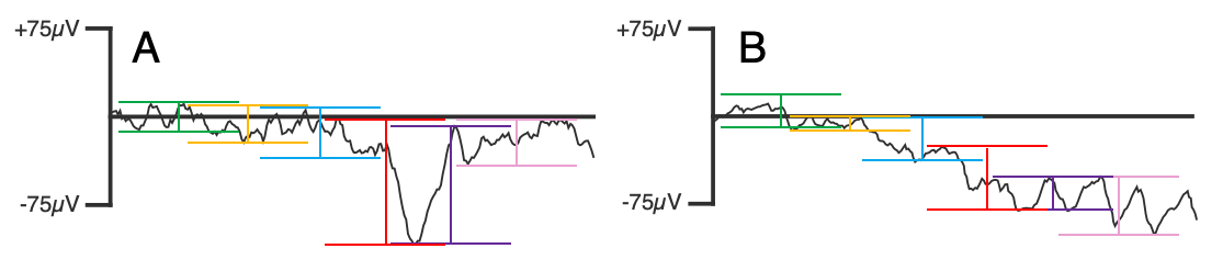
The first is called the moving window peak-to-peak algorithm, and it’s illustrated in Figure 8.3. With its default parameters and our epochs of -200 to 800 ms, this algorithm will start by finding the difference in amplitude between the most positive and most negative points (the peak-to-peak voltage) between -200 and 0 ms (a 200-ms window). Then, the window will move 100 ms to the right, and the algorithm will find the peak-to-peak voltage between -100 and 100 ms. The window will keep moving by 100 ms, finding the peak-to-peak amplitude from 0 to 200 ms, 100 to 300 ms, etc. It then finds the largest of these peak-to-peak amplitudes for a given epoch and compares that value to the rejection threshold.
Figure 8.3.A illustrates the application of this algorithm to a trial with a blink. You get a large peak-to-peak amplitude during the period of the blink because of the relatively sudden change in voltage. However, the algorithm isn’t “fooled” by the slow drift shown in Figure 8.3.B.
Figure 8.3. Moving window peak-to-peak algorithm. The peak-to-peak amplitude is determined in each window, and then the maximum of these values for a given epoch is compared with the rejection threshold.
Let’s try it. Go back to 1_MMN_preprocessed_interp_be as the active dataset and select EEGLAB > ERPLAB > Artifact detection in epoched data > Moving window peak-to-peak threshold. Set the window width to 200 ms and the window step to 100 ms (so that we get a 200-ms window every 100 ms). Set the threshold to 100 and the channel to 33 (VEOG-bipolar). Click ACCEPT to run the routine.
The first thing to note is that 28.2% of trials have been flagged for rejection. That’s a lot more than we had with the absolute voltage threshold; we’ll discuss the reasons for that in a moment.
If you scroll through the data, you’ll see that every clear blink has now been flagged (including Epochs 104 and 170, which were missed by the absolute threshold algorithm). However, more trials with muscle noise have now been flagged for rejection. Here’s why: Imagine that the muscle noise causes the voltage to vary from -55 to +55 µV between 200 and 400 ms. This doesn’t exceed the absolute threshold of ±100 µV, but it creates a peak-to-peak amplitude of 110 µV, exceeding our threshold for the peak-to-peak amplitude. One way to solve this would be to increase the threshold to something like 120 µV. However, this would cause us to start missing real blinks.
Another approach would be to apply a low-pass filter prior to artifact detection. Let’s give that a try. Go back to 1_MMN_preprocessed_interp_be as the active dataset and select EEGLAB > ERPLAB > Artifact detection in epoched data > Moving window peak-to-peak threshold. Keep the parameters the same, but check the box labeled Low-pass prefiltering… and set the Half-amplitude cutoff to 30. This option creates a hidden copy of the dataset, applies the filter to it, and applies the artifact detection algorithm to this hidden copy. The artifact detection flags are then copied to the original dataset. That way, you get the benefits of prefiltering the data in terms of flagging appropriate trials, but you end up with your original unfiltered data.
Click Accept to run the artifact detection routine. You’ll see that only 13.0% of trials are flagged for rejection (compared to 28.2% without prefiltering). If you scroll through the data, you’ll see that all the clear blinks are flagged, but the trials with EMG noise are not. If you check the data quality measures using EEGLAB > ERPLAB > Compute data quality metrics (without averaging), you’ll see that the aSME for FCz has improved slightly relative to the rejection based on the absolute voltage threshold. And if you plot the ERP waveforms, you’ll see that they’re quite similar to what we found with the absolute voltage threshold.
So, the moving window peak-to-peak algorithm is definitely superior to the absolute voltage threshold algorithm. It doesn’t make a huge difference with this participant, but it makes a big difference for some participants and some experimental paradigms. However, in many cases, you’ll want to use the low-pass prefilter option.
Now let’s look at another algorithm that works quite well but doesn’t require any low-pass filtering. I call this algorithm the step function, because I developed it to detect the step-shaped voltage deflections produced by saccadic eye movements in N2pc paradigms. I eventually discovered that it also works great for detecting blinks.
The step function also involves a moving window, with 200 ms as a reasonable default value for most studies. Within a 200-ms window, this algorithm calculates the difference between the mean voltage in the first half of the window and the mean voltage in the second half of the window. It then finds the largest of these differences for all the windows in a given epoch, and it compares the absolute value of this difference to the rejection threshold. For example, the window indicated by the red lines in Figure 8.3.A has an amplitude of approximately 20 µV during the first half and approximately 70 µV during the second half, so this would be a difference of approximately 50 µV. That wouldn’t exceed a threshold of 100 µV, but you can use a lower threshold with the step function than with the other algorithms. Also, you will get the largest voltage from a blink if the center of the window is just slightly before the start of the blink, and a smaller step size (e.g., 10 ms) tends to be better.
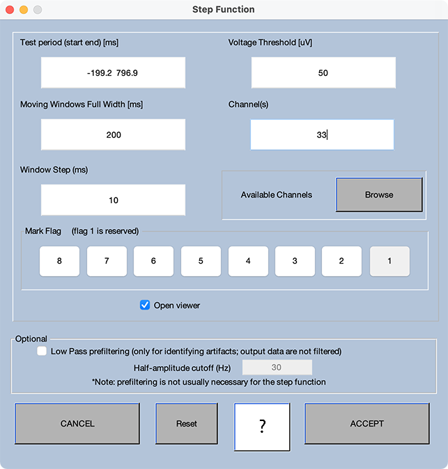
Let’s try it. Go back to 1_MMN_preprocessed_interp_be as the active dataset and select EEGLAB > ERPLAB > Artifact detection in epoched data > Step-like artifacts. Set the parameters as shown in Screenshot 8.3. Specifically, set the window width to 200 ms and the window step to 10 ms (so that we get a 200-ms window every 10 ms). Set the threshold to 50 µV and the channel to 33. Click ACCEPT to run the routine.
Screenshot 8.3
You should first note that 13.1% of trials have been flagged for rejection, which is nearly identical to what we obtained when we used the moving window peak-to-peak algorithm with the prefiltering option. But note that no filtering is required with the step function: when the step function algorithm averages across each half of the 200-ms window, high-frequency activity is virtually eliminated.
If you scroll through the EEG, you’ll see that the algorithm has successfully flagged all of the clear blinks without flagging many non-blink trials. In my experience, the step function works slightly better than the moving average peak-to-peak algorithm (especially when there is a lot of EMG noise) and significantly better than absolute voltage thresholds. It’s what I recommend for detecting blinks in most cases.