When deciding on artifact rejection parameters, a key question is whether the data quality will be increased or decreased by making the rejection threshold more liberal (rejecting fewer trials) or more conservative (rejecting more trials). We can answer that question quantitatively by looking at the SME values that result from different rejection parameters. However, we also need to determine whether the artifacts are creating confounds, which involves inspecting the averaged ERP waveforms in several ways. In this exercise, we’ll go through the steps needed to check both the data quality and the waveforms.
Let’s start by looking at the SME values and waveforms that we get without any rejection. Select the dataset with the ±100 µV threshold (1_MMN_preprocessed_interp_be_ar100) and then select EEGLAB > ERPLAB > Compute averaged ERPs. Near the top of the averaging GUI, select Include ALL epochs (ignore artifact detections). This will allow us to see what we would get without any artifact rejection. As described in the preceding chapter, select On – custom parameters in the Data Quality Quantification section and add a time window of 125 to 225 ms (the time window we will ultimately use to measure MMN amplitude). Click RUN, and name the resulting ERPset 1_ar_off.
If you look at the data quality table, you’ll see that the aSME at FCz during the custom time period of 125-225 ms is 0.5524 for the deviant stimuli (Bin 1) and 0.3641 for the standards (Bin 2). (Leave the data quality window open for comparison with later steps.)
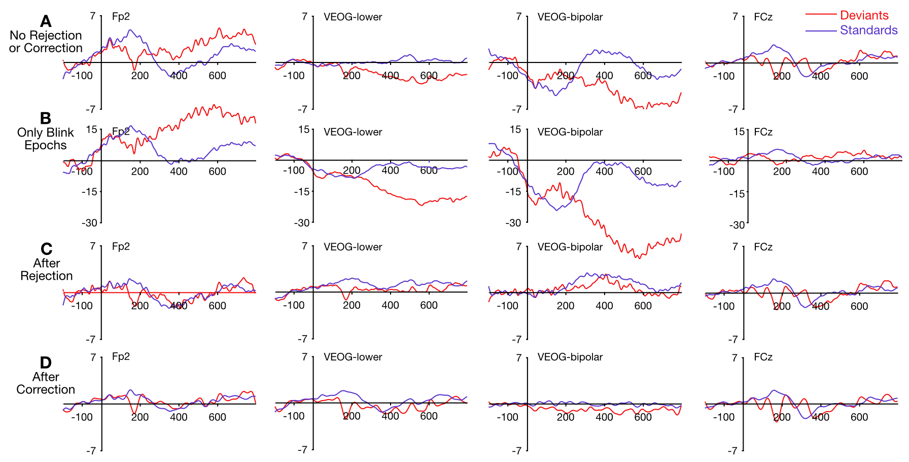
Now plot the ERP waveforms. You can see some relatively large, slow deviations in the Fp2, VEOG-lower, and VEOG-bipolar channels. The key channels are shown in Figure 8.2.A, but I’ve applied a 20 Hz low-pass filter to more easily see the blink-related activity. If you look closely at the FCz channel, which will be the primary channel for our MMN analyses, you can see some of this same blink-related activity (i.e., the “tilt” in the prestimulus period).
Figure 8.2. Averaged ERPs from Subject #1 in the MMN experiment, with no rejection or correction (A), including only epochs flagged for blinks (B), after rejection of epochs with blinks using an absolute voltage threshold of ±100 µV (C), and after ICA-based correction of blinks (D). To improve visualization of the data, the averaged waveforms were low-pass filtered with a half-amplitude cutoff at 20 Hz and a slope of 12 dB/octave. Note the different scale in (B).
Are the large, slow voltage deviations in Figure 8.2.A a result of blinks that are confounding the ERPs, or are they brain activity? One way to answer this question is to look for a polarity reversal under versus over the eyes. The activity prior to ~200 ms is more negative for deviants than for standards both under the eyes (VEOG-lower) and above the eyes (Fp2), so this experimental effect is probably not blink-related. However, the later voltage is more negative for deviants than for standards under the eyes but more positive for deviants than for standards above the eyes. This polarity inversion is suggestive of a blink confound (although it is possible for brain-generated activity to invert in polarity above versus below the eyes).
Another way to address this question is to reverse the usual artifact rejection procedure and include only the flagged trials in our averages, leaving out the unflagged trials. Any blink-related confounds should be much bigger in these averages, whereas brain activity should not. To do this, run the averaging tool again, but this time select Include ONLY epochs marked with artifact rejection. If you look at the resulting waveforms, you’ll see that the differences between deviants and standards prior to ~200 ms are about the same as before, but the differences after 200 ms are now much larger (see Figure 8.2.B). This provides additional evidence that the participant was more likely to blink following deviant stimuli than following rare stimuli (even though the auditory stimuli were task-irrelevant). Thus, blinking is not just a source of noise in this experiment; it's a confound that could create artifactual differences between conditions during the latter part of the epoch.
Now let’s look at the data quality and waveforms when we reject trials that were flagged for blinks. You can just repeat the averaging process, but select Exclude epochs marked during artifact detection so that the flagged epochs are excluded. If you keep the previous table of data quality values open, and open a new table for the current ERPset, you’ll see that the aSME at FCz from 125-225 ms has dropped from 0.5524 to 0.5436 for the deviant stimuli and from 0.3641 to 0.3377 for the standards. We have fewer trials as a result of artifact rejection, but the data quality has improved. The improvement isn’t very large, because we now have fewer trials and because the blinks that we’ve removed are not huge at the FCz site. But it’s still good to see that we get better data quality even though we have fewer trials in the averages. (There is a much larger improvement in data quality at Fp1 and Fp2, where the blinks were a large source of trial-to-trial variation.)
Even though rejecting epochs with blinks hasn’t improved our data quality much, at least it hasn’t hurt our data quality. And rejecting blinks helps us avoid blink-related confounds: if you plot the waveforms, you’ll see that we’ve reduced the slow voltage deviations in the VEOG, Fp2, and FCz channels. You can see this quite clearly in Figure 8.2.C, where the voltage deviations are now reduced relative to the no-rejection data shown in Figure 8.2.A. You can see substantial differences between the standards and the deviants in the VEOG-bipolar channel in the absence of artifact rejection, which suggests that the blinks were not random and differed systematically between trial types. These difference are largely eliminated by artifact rejection.
As described at the beginning of the chapter, artifact rejection is designed to deal with three specific problems: reduced statistical power, systematic confounds, and sensory input problems. The artifact rejection procedure that you’ve performed has achieved the first two of these goals: you’ve slightly reduced the noise (as evidenced by the lower aSME values) and thereby increased the statistical power, and you’ve minimized a confound (differential blink activity between standards and deviants).
Figure 8.2.D shows the results with ICA-based correction of blink artifacts (which will be covered in the next chapter). You can see that this approach eliminated blink-related activity better if you look at the VEOG-bipolar channel, which largely isolates blink-related activity. This channel is nearly flat in the corrected data but not in the rejected data. However, the corrected and rejected waveforms look nearly identical at the FCz site—which is what we really care about—except that the rejected waveforms are noisier because we’ve lost some trials in the rejection process. This shows that rejection is working reasonably well: We’re eliminating confounding activity from the blinks without a huge reduction in data quality. However, the waveforms appear to be cleaner for the corrected data (because we’ve retained all the epochs), and I confirmed this by computing SME values (which were 0.4992 for the deviants and 0.2815 for the standards). Because of this better data quality, I usually prefer ICA-based artifact correction instead of rejection for blinks. However, we still reject trials with blinks that occur near the time of the stimulus in visual experiments, because we want to exclude trials on which the participant could not see the stimulus.
An important take-home message of this exercise is that artifact rejection is designed to address three specific problems, and you want to choose the parameters that best solve these problems. You can assess data quality and statistical power by examining the SME values. You can assess confounds by looking for polarity inversions above versus below the eyes in the averaged ERP waveforms. It also helps to view the waveforms for averages of all epochs, averages of just the epochs with artifacts, and averages that exclude epochs with artifacts. Blinks and eye movements don’t create obvious problems with the sensory input in most auditory paradigms, but we will see how they impact a visual paradigm near the end of the chapter.