Our first attempt at ICA-based blink correction was quite simplistic, and as a result the decomposition was not very good (as evidenced by the irregularly shaped scalp maps for some of the ICs in Screenshot 9.2). The main reason for this is that our dataset (like most EEG datasets) contains some really large activity that is difficult for ICA to handle because it is either infrequent or lacks a consistent scalp distribution (e.g., skin potentials). In this exercise, we’ll look at an approach that will minimize the effects of those large noise sources and also make the decomposition run faster. It’s a win-win!
There are several steps for making the ICA decomposition work better. Some of them are based on a trick, which is to create a new dataset in which we’ve removed signals that will be problematic for ICA, do the decomposition on this new dataset, and then transfer the ICA weights back to the original dataset. This approach was controversial when I wrote my other book, so I didn’t recommend it in Chapter 6 of Luck (2014). However, the field has largely converged on the idea that this approach is both theoretically justified and practically useful.
The first thing we’re going to do is heavily filter the data, using filter settings that I would never ordinarily use for ERP experiments. However, the filtered data will be used only to do the ICA decomposition, and then we’ll transfer those ICA weights to the original data.
Why Heavy Filtering is OK for the ICA Decomposition
Filters change the time course of an underlying IC, but not the scalp distribution, Heavy filtering is therefore fine for the data used for the ICA decomposition, because we only care about scalp distributions at this stage, not the timing. Once we have the IC weights, we’ll transfer them back to the original data without the temporal distortion caused by the filtering.
To get started, quit and restart EEGLAB and then load the original dataset for Subject 10 (10_MMN_preprocessed). Select EEGLAB > ERPLAB > Filter & Frequency Tools > Filters for EEG data, specifying a high-pass cutoff of 1 Hz and a low-pass cutoff of 30 Hz, with a slope of 48 dB/octave. Run the routine and save the resulting dataset as 10_MMN_preprocessed_filt. We’ve now eliminated most of the skin potentials and EMG, both of which may violate the assumptions of ICA and interfere with the decomposition.
Our next step is to downsample the data to 100 Hz. This just makes the ICA decomposition run faster (as does the reduction of noise produced by the filtering). To do this, select EEGLAB > Tools > Change sampling rate, enter 100 as the new sampling rate, and then name the resulting dataset 10_MMN_preprocessed_filt_100Hz.
The next thing we’re going to do to improve ICA is remove the segments of data during breaks, when the participants may be moving, scratching their heads, chewing, etc. The voltages produced by these actions are typically large but don’t have a consistent scalp distribution. EEGLAB allows you to manually select and delete these time periods from a continuous dataset. ERPLAB adds an automated procedure for this. It just finds periods of time without any event codes and deletes them. Let’s give it a try.
Select EEGLAB > ERPLAB > Preprocess EEG > Delete Time Segments (continuous EEG). In the window that appears, specify 1500 as the Time Threshold. This tells the routine to delete segments in which there are no event codes for at least 1500 ms. The event codes in the MMN experiment occur every ~500 ms, so periods of 1500 ms without an event code must be breaks. Of course, you’d need to use a longer value for experiments with a slower rate of stimuli. Also specify 500 as the amount of time prior to the first event code in a block of trials. This will make sure that we have at least 500 ms for the prestimulus baseline period for the first event in a trial block. Similarly, specify 1500 ms as the time period after the last event code in a block so that we have a good period of data following this event code.
Enter 1 in the field for Eventcode exceptions. This tells the routine to ignore this event code. Our stimulus presentation program sent some event codes with a value of 1 during the breaks, and we want those to be ignored when looking for break periods. Similarly, check the box for ignoring boundary events. Boundary events occur whenever there is a temporal discontinuity in the data. Most commonly, this happens when you have a separate data file for each block and then concatenate them together into a single file. When you do this, a boundary event is inserted at the time point of the transition between one block and the next. Boundary events often occur during breaks, so we want them to be ignored when we’re looking for long periods between event codes. Make sure the Display EEG button is checked and click RUN.
You’ll then see two new windows, one for displaying the EEG dataset and one for saving the new dataset. If you scroll through the data, you’ll see a red background for the first ~25 seconds and the last ~3 seconds, which are the break periods at the beginning and end of the trial block (we have only one trial block in this experiment). These are the time periods that will be deleted. You should always verify that it worked correctly, and then you can save the new dataset as 10_MMN_preprocessed_filt_100Hz_del.
Finally, we’re going to deal with bad channels. F7 and PO4 both show some crazy behavior in this dataset. If we leave them in the data, we’ll end up with an IC that just represents F7 and another that just represents PO4. In fact, you can see this in our original ICA decomposition in Screenshot 9.2, where IC 3 just represents the F7 channel and IC 17 just represents the PO4 channel. We’re going to interpolate these channels eventually, so why include them in the ICA decomposition? We could interpolate them prior to the ICA decomposition, but that might create a linear dependency among the channels that would mess up the decomposition. Instead, we’ll just exclude them from the ICA decomposition process, and then we can interpolate them after artifact correction is complete.
Now let’s apply the ICA decomposition to this dataset by selecting EEGLAB > Tools > Decompose data by ICA. We’re going to exclude Channels 3 and 24 (the channels for F7 and PO4, respectively), and we’re also going to exclude Channels 32 and 33 (the bipolar EOG channels). To do this, type 1 2 4:23 25:31 into the Channel type(s) or indices field. As before, make sure to use runica as the ICA algorithm and that 'extended', 1 is specified in the field for options (see the EEGLAB ICA documentation for an explanation of this option). Then run the routine. If you don’t want to wait for it to finish, you can just load the dataset I created after running the decomposition, named 10_MMN_preprocessed_filt_100Hz_del_ICAweights.
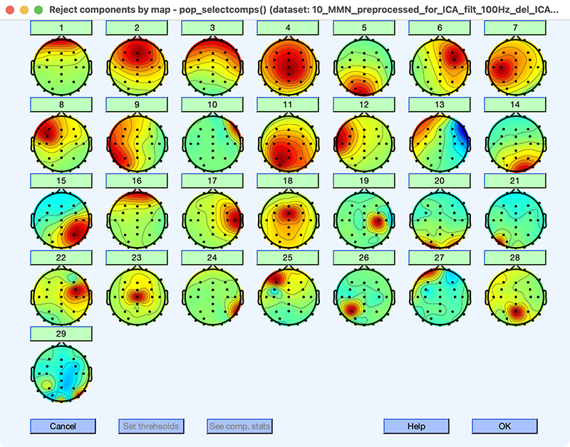
Once you have the weights, you can view the results with EEGLAB > Tools > Inspect/label components by map. The result I obtained in shown in Screenshot 9.6 (your results may differ slightly, especially the ordering and polarity of the ICs). These maps are much nicer than our original maps (Screenshot 9.2). Almost all have either a single focus with a largely monotonic decline (e.g., IC 1 and IC 2) or a bipolar configuration (e.g., IC 13 and IC 15). IC 20 has two foci that are approximately mirror-symmetric across the left and right hemispheres, which is also a perfectly normal pattern (and arises when the two hemispheres operate synchronously). The only irregular map is for IC 29. Because the maps are ordered according to the amount of variance they explain, you shouldn’t worry if the last couple of maps aren’t perfect.