Our goal in heavily filtering the data was to improve the ICA decomposition, but as was described in the chapter on filtering, this kind of filtering is usually a bad idea for ERP analyses. So, we’re going to take our optimized ICA decomposition and transfer the weights to the original dataset, which has not been distorted by filtering. To do this, first look at the Datasets menu in EEGLAB and note the dataset number for the dataset containing the ICA weights (10_MMN_preprocessed_filt_100Hz_del_ICAweights). It’s probably #4, but it might be something else if you’ve done some other processing. Now select the original dataset (10_MMN_preprocessed) in the Datasets menu and then select EEGLAB > Edit > Dataset info. In the new window that appears, click the From other dataset button for the ICA weights array, and enter the number for the dataset with the ICA weights (probably 4). Also change the Dataset name to 10_MMN_preprocessed_transferredICAweights, and then click OK. That’s it! You’ve now transferred the weights. You might want to save this dataset to your disk with EEGLAB > Files > Save current dataset as.
You can verify that the weights have been transferred by selecting EEGLAB > Tools > Inspect/label components by map (but first close the window you created with this routine in the previous exercise, if it’s still open). You should see the same maps as in the previous exercise (Screenshot 9.6), because you transferred those weights to the current dataset.
Now let’s compare the time course of the ICs (EEGLAB > Plot > Component activations (scroll)) with the time course of the EEG and EOG data (EEGLAB > Plot > Channel data (scroll)). You can see that the time course of IC 1 closely matches the time course of the blinks and vertical eye movements in VEOG-bipolar. To the naked eye, there isn’t any obvious difference between IC 1 from this decomposition and IC 1 from our original decomposition (Screenshots 9.2-9.4). However, given that the decomposition as a whole improved, IC 1 from our new decomposition is less likely to be contaminated by activity from other sources (less lumping).
Now let’s see if we can figure out what’s going on with the other ICs and see if any of them should be removed along with IC 1. Let’s start by looking for an IC related to horizontal eye movements. Go back to the plot of the scalp maps (Screenshot 9.6) and see if any of the maps have the distribution you’d expect for horizontal eye movements (i.e., opposite-polarity foci just to the sides of the two eyes). IC 13 looks promising, so click on the 13 above the scalp map for IC 13 (or the IC that has the right scalp distribution if your maps don’t exactly match Screenshot 9.6). A new window will pop up to show the details of this IC. The time course heatmap has a lot of activity at the beginning and end of the dataset, which is what we would expect if large eye movements were most common during the break periods at the beginning and end of the session. (Note that we deleted the break periods in the dataset used for the ICA decomposition, but we’ve now transferred the weights to the original dataset, which still has data during the break periods. The same set of weights is used for every time point, so it’s not a problem to transfer weights to time points that weren’t used in the ICA decomposition.)
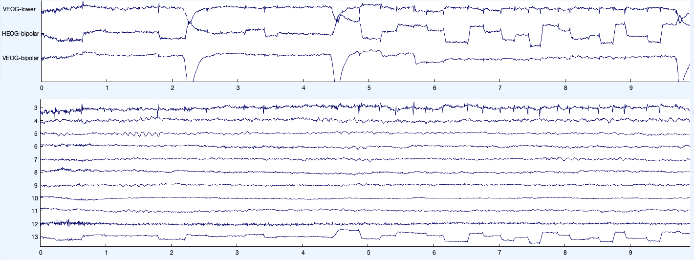
Now go back to the scrolling time course plots for the ICs and EEG data and see if the time course of IC 13 matches the time course of the horizontal eye movements in HEOG-bipolar. You might want to display only 6 channels and ICs at a time so that you can see the eye movements better. Screenshot 9.7 shows the EOG data (top) and a few of the ICs (bottom) for the first 10 seconds of the dataset. You can see a beautiful correspondence between IC 14 and HEOG-bipolar. And if you look closely at the other ICs, none of them show the same pattern. ICA has clearly done a good job of isolating the horizontal eye movements with IC 13. We should definitely consider removing IC 13 from the data.
Screenshot 9.7
Although none of the other ICs show the same pattern as the HEOG-bipolar channel, IC 3 has a sharp voltage spike at the onset time of each shift in eye position. This is the spike potential shown in Figure 9.1, which is the muscle contraction that causes the eyes to move. Given that the spike potential and the change in HEOG voltage are closely linked, you might wonder why they end up in different ICs. The answer is that ICA tries to find ICs that are maximally independent at a given time point. The HEOG signal is sustained, and the spike potential occurs only at the very beginning of the eye movement, so you often have a large HEOG voltage with no spike potential. And the spike potential slightly precedes the HEOG change, so you can have a large spike potential with HEOG. Consequently, they end up as different ICs. Note that the magnitude of the spike potential in the EEG/EOG recordings varies considerably across participants, so you don’t always see a separate IC for it.
IC 4 has a midline centro-parietal focus and a broad scalp distribution, much like the P3b wave. However, the participants weren’t doing a task in the MMN experiment, so we wouldn’t expect to see the P3b. If you scroll through the component activations and EEG data, it’s hard to see any obvious correspondence between IC 4 and the EEG signals. Moreover, the power spectrum doesn’t reveal a clear peak, so it doesn’t seem to be an oscillation. I really don’t know what IC 4 is.
IC 5, on the other hand, shows a clear peak at 10 Hz (which you can see by clicking on the 5 above the scalp map for IC 5). Also, the scalp map has a strong focus at the occipital pole. Both of those are consistent with the classic alpha-band oscillation first described by Hans Berger in his original EEG study (Berger, 1929). You can see some beautiful alpha bursts in both IC 5 and the posterior EEG electrodes between 57 and 60 seconds.
IC 2 also has a clear peak in its power spectrum, but at approximately 7 Hz instead of 10 Hz. Its scalp map has a focus around Fz. Given this power spectrum and scalp topography, this is probably the commonly-observed midfrontal theta oscillation. You can see bursts of oscillatory activity in this IC at a variety of time points (e.g., 127-128 s, 219 s, 297-302 s, 401-403 s), and you can see corresponding bursts of oscillations in the far frontal channels. However, the oscillation bursts sometimes occur simultaneously in other ICs (e.g., at 127 s), and IC 2 also shows some transient (non-oscillating) activity, so I wouldn’t try to use this IC to isolate midfrontal theta and then use it as a dependent variable.
Check out the rest of the ICs and see if you can figure out what they represent. You’ll see that some contain alpha-band activity, like IC 5, but with somewhat different scalp topographies. This isn’t surprising given that alpha can be observed over different cortical areas at different times. Many ICs have no obvious interpretation. IC 16 has a scalp distribution that is much like IC 1. Blinks often appear in two or even three ICs, so you should take a close look at any IC that has a blink-like scalp map.
If you scroll through the component activations and EEG/EOG data, you’ll see that IC 16 exhibits a high-frequency burst at the beginning of each blink, superimposed on a negative dip. This could be the EMG activity from the muscles that produce the blink. However, the slower negative dip doesn’t seem like EMG, so IC 16 may be mixing EMG and EOG signals. It’s still blink-related, so we’ll consider whether to exclude it in the next exercise.
Blink-related EOG activity is primarily a result of the eyelids sliding across the eyeballs, but there may also be a slight vertical rotation of the eyeballs that produces a voltage. These two effects have similar but slightly different scalp distributions, so they may appear as separate ICs (especially when you have 60 or more channels and therefore 60 or more ICs). In theory, the two eyelids could start and stop moving at slightly different times, which might also produce separate ICs.