So far, we’ve been measuring and analyzing the data only from the C3 and C4 channels, where the LRP is largest. However, it’s often valuable to include the data from multiple channels. One way to do that is to measure from multiple different channels and include channel as a factor in the statistical analysis. However, that adds another factor to the analysis, which increases the number of p values and therefore increases the probability of getting bogus-but-significant effects. Also, interactions between an experimental manipulation and electrode site are difficult to interpret (Urbach & Kutas, 2002, 2006). In most cases, I therefore recommend averaging the waveforms across the channels where the component is large, creating a cluster, and then obtaining the amplitude or latency scores from the cluster waveform. Averaging across channels in this manner tends to produce a cleaner waveform, which decreases the measurement error (as long as we don’t include channels where the ERP effect is substantially smaller). Also, it avoids the temptation to “cherry-pick” the channel with the largest effect.
In the ERP CORE flankers experiment, the LRP effect was only slightly smaller in the F3/F4 and C5/C6 channels than in the C3/C4 channel, so we should be able to decrease our measurement error and increase our effect sizes by creating a cluster of these three sets of channels.
I’ve already created this cluster in the difference waves in the Chapter_10 folder. They’re in Channel 12, which is labeled cluster. Let’s try measuring the peak latency from this channel in the filtered data (which should already be loaded). You can just repeat the measurement and analysis procedures from the earlier exercise where we measured the peak latency from the filtered data, but changing the Channel from 5 to 12. You should see that the effect size has increased a bit (-0.683 for the cluster analysis relative to -0.630 when we measured from the C3/C4 channel). Collapsing across channels doesn’t always increase the effect size, but it doesn’t usually hurt, and it avoids the need to include channel as a factor in the analysis or the need to determine which one channel to use. My lab now measures from a cluster in virtually all of our studies.
Our last step will be to ask whether the peak latency values are correlated with response times (RTs). That is, do participants with later LRP peaks also have slower RTs? Unfortunately, it takes some significant work to extract RTs using ERPLAB. In your own experiments, you might want to do this using the output of your stimulus presentation system instead of using ERPLAB. For the present exercise, I wrote an ERPLAB script to obtain the mean RTs for Compatible and Incompatible trials for each participant. I saved the values to an Excel spreadsheet named RT.xlsx, which you can find in the Chapter_10 folder. An advantage of using an ERPLAB script to get the RTs is that you can exclude the trials that were rejected because of artifacts from the mean RTs so that the ERP data and the behavioral data are based on exactly the same set of trials. A disadvantage is that it takes a bit of work. I’ve provided the script I wrote for this purpose (named get_LRP_RTs.m in the Chapter_10 folder), which you can use as a model for your own studies.
Let’s look at the correlations. You’ll need to combine the RT values from the spreadsheet with the peak latency values that you just created from the waveforms that were collapsed across the three pairs of electrode sites. And then you’ll need to read them into your statistical package or into a spreadsheet program (see peak_latency_filt_collapsed.xlsx in the Chapter_10 folder). You’ll then want to look at the correlation between peak latency and RT separately for the Compatible condition and the Incompatible condition.
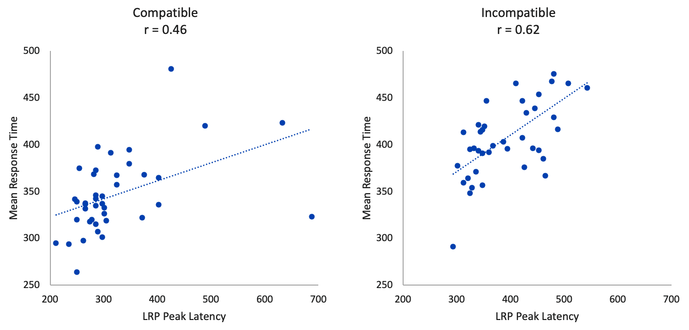
Figure 10.5 shows the results I obtained in Excel. The peak latency scores were correlated fairly well with the RTs, especially for the incompatible trials. Some outliers in the LRP peak latency scores for the Compatible trials clearly reduced the correlation in the that condition. Nonetheless, these correlations show that the timing of the brain activity is related to the timing of the behavioral response.
Figure 10.5. Scatterplots showing the relationship between LRP peak latency and response time for the Compatible and Incompatible conditions.