As described in Chapter 2 of Luck (2014), the onset time of a difference between two conditions can be extremely informative. For example, the brain can’t have a more negative response over the contralateral hemisphere than over the ipsilateral hemisphere until it has determined which hand should respond, so the onset latency of the LRP can be used as a marker of the time at which the brain has decided on a response (see Chapters 2 and 3 in Luck, 2014, for a more detailed and nuanced discussion).
How can we quantify the onset time of a difference wave? Consider, for example, the Compatible waveform in Figure 10.2.C. The negativity of the LRP first falls below the zero line a little before 200 ms. However, the negativity before 200 ms is no larger than the noise level (as assessed, e.g., by the variations in voltage during the prestimulus period). Early research attempted to solve this problem by using a statistical criterion such as the first of N consecutive points that are at least 2 standard deviations greater than the noise level (where the standard deviation is measured from the variation in voltage during the prestimulus period). However, this approach suffers from low power, and single-participant scores will vary according to the noise level as well as the true onset time. A terrific study by Kiesel et al. (2008) rigorously compared this technique with peak latency and two other measures that were not very widely used at the time—fractional area latency and fractional peak latency—and found that the two less widely used scoring methods were actually the best. These two methods are now more commonly used, and we’ll focus on them here.
We already looked at fractional area latency in the previous exercise, but we used it to estimate the midpoint latency (the 50% area latency) rather than the onset latency. To estimate the onset latency, we simply need to use a lower percentage. In the present exercise, we’ll calculate the time at which the area reaches the 15% point. To get started, make sure that the 40 ERPsets from the Chapter_10 > Data > ERPsets_CI_Diff folder are loaded. Launch the Measurement Tool, and set it up as in the previous exercise (Screenshot 10.7), except change the percentage from 50 to 15, and change the name of the output file to something like FAL15_latency.txt. Take a look at the scores for the individual waveforms using the Viewer, and then run the measurement routine to save the scores.
As before, load the resulting scores into your statistical package and compute the paired t test to compare the Compatible and Incompatible conditions. You should see that difference in means across conditions is ~50 ms and that the effect is statistically significant (t(39) = -6.06, p < .001) with a very large effect size (d = -1.044).
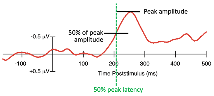
Now let’s try the other scoring algorithm, fractional peak latency, which is illustrated in Figure 10.4. This method finds the peak and then moves backward in time until the voltage reaches some fraction of the peak voltage (usually the 50% point). The latency of this point is then used as the estimate of onset latency. You might wonder why we usually choose the 50% point. Isn’t the 15% point, for example, closer to the true onset? There are two reasons to choose the 50% point. First, it’s less influenced by noise and therefore more reliable than lower percentages. Second, it actually does a better job of capturing the average onset time given that there is almost always significant trial-to-trial variation in onset times. As discussed in Chapter 2 of Luck (2014), the first moment that an averaged waveform deviates from zero is driven by the trials with the earliest onset times. And as discussed in Chapter 9 of that book, the 50% peak latency point accurately captures the average of the single-trial onset times under some conditions.
Figure 10.4. Example of the fractional peak latency method. In this example, we obtained the 50% peak latency (the latency at which the voltage reached 50% of the peak voltage).
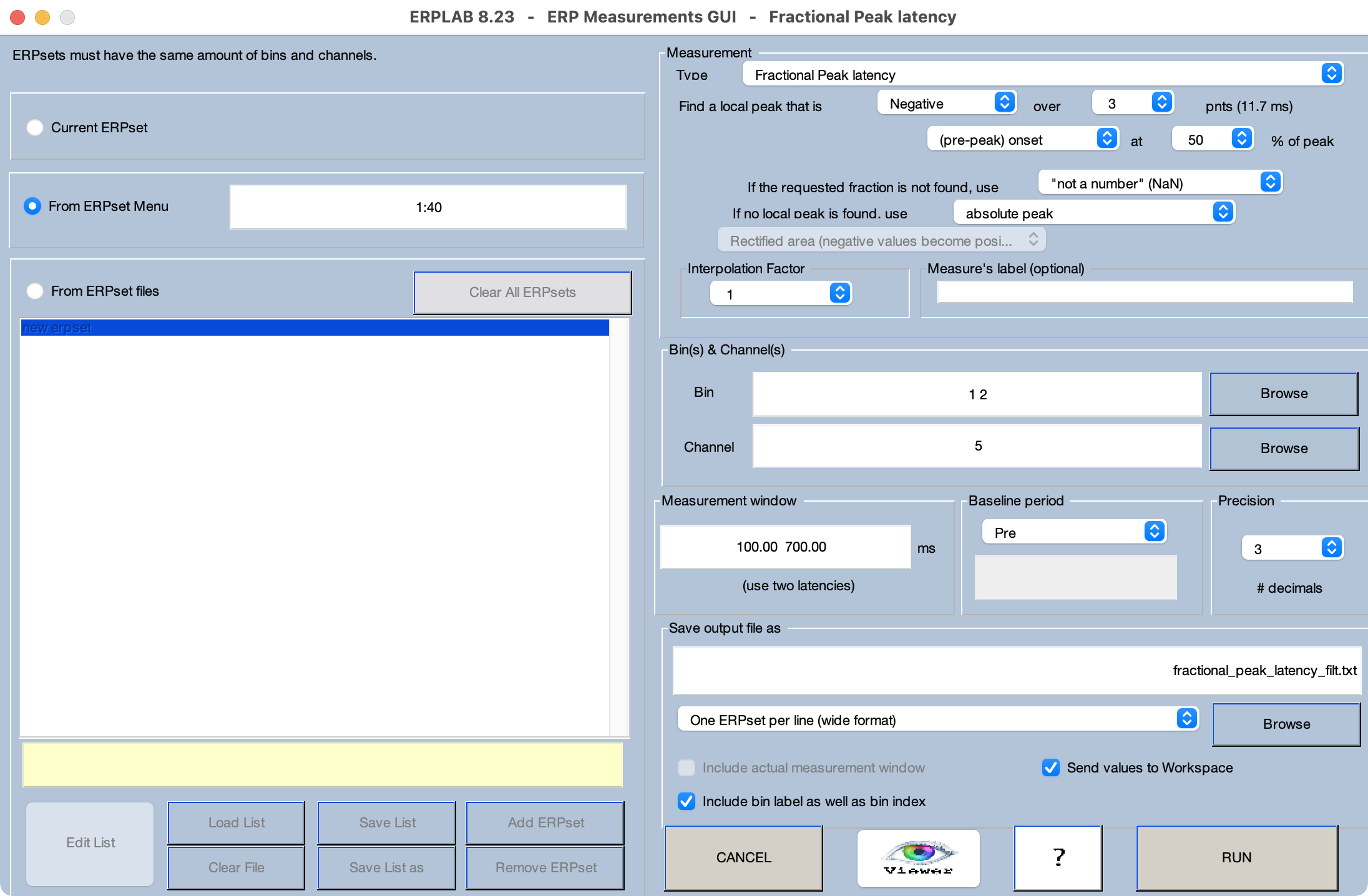
Let’s give it a try. First, clear the existing ERPsets out of ERPLAB (or quit and restart EEGLAB) and load the filtered ERPsets in the Chapter_10 > Data > ERPsets_CI_Diff_filt folder. This scoring method is, unfortunately, very sensitive to high-frequency noise, so we ordinarily apply fairly aggressive low-pass filtering (which, fortunately, has relatively little impact on the 50% peak latency). Launch the Measurement Tool, and set it up as shown in Screenshot 10.8. Once you have the parameters set, use the Viewer to make sure that the scores look appropriate for the single-participant waveforms. Then run the routine to save the scores to a file named fractional_peak_latency_filt.txt.
Screenshot 10.8
Load the resulting scores into your statistical package and compute the paired t test. You should see that difference in means across conditions is ~50 ms, just as for the 15% area latency measure from the previous exercise. The effect is statistically significant (t(39) = -4.39, p < .001), but the effect size is smaller than observed in the previous exercise (d =-0.695 for 50% peak latency versus d = -1.044 for 15% area latency).
So, which of these two scoring methods is best? The effect size was larger for 15% area latency than for 50% peak latency in the analysis you just did. Also, Kiesel et al (2008) found that 50% area latency yielded less variability than 50% peak latency. Unfortunately, they didn’t examine 15% area latency, and they didn’t apply an aggressive low-pass filter prior to obtaining the 50% peak latency scores. We also found lower standard deviations for 50% area latency than for 50% peak latency for all of the basic difference waves in the six ERP CORE paradigms (see Table 3 in Kappenman et al., 2021). However, the 50% area latency captures the midpoint of the difference wave, not the onset, which is less sensitive to noise, so this really isn’t a fair comparison. I think it’s fair to say that this issue is unresolved at this point.
However, there is an important conceptual difference between these two scoring methods. Specifically, fractional area latency is impacted by voltages throughout the entire measurement window. For example, the negative voltage late in the waveform for the Incompatible trials (see Figure 10.2.C) will have an impact on the 15% fractional area latency score. By contrast, fractional peak latency is not influenced by anything that happens after the peak. This is particularly clear in the example shown in Figure 10.4, where there is a long “tail” to the difference wave that will have a large impact on the fractional area latency score but will have no impact on the fractional peak latency score. For this reason, I usually use the fractional peak latency score.
This exemplifies a broader issue: Although minimizing measurement error is important, it’s also important to make sure that your scoring method is valid (i.e., measures what you are trying to measure with minimal influence from other factors).