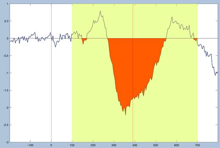
In this exercise, we’re going to look at a different latency scoring algorithm called fractional area latency, which is often superior to peak latency (especially when measured from difference waves). For a negative component like the LRP, this algorithm calculates the area of the waveform below the zero line and then finds the time point that divides the area into two areas at a particular percentage. If you want to estimate the midpoint of the waveform, you will look for the 50% point (the time that divides the area into two equal halves). This is then called the 50% area latency (see Chapter 9 in Luck, 2014, for more details). Screenshot 10.6 shows what it looks like when I apply this algorithm to Bin 2 (Incompatible) from the grand average, using a measurement window of 100 to 700 ms. The area under the curve in this measurement window is shaded in red, and the point that divides this area into two equal halves is indicated by the red vertical line. This region includes some little areas near the beginning and end of the measurement window, but that’s just how it goes. It’s difficult to perfectly quantify ERP amplitudes and latencies, and we have to live with some error.
Screenshot 10.6
Don’t Worry About High-Frequency Noise in Area-Based Measures
Area-based measures like fractional area latency are relatively insensitive to high-frequency noise, so we will apply this method to the unfiltered data. It's also usually unnecessary to filter out high-frequency noise when measuring mean amplitude.
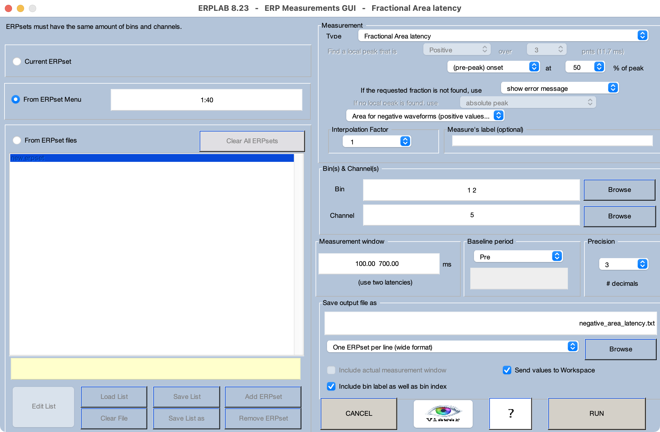
Let’s apply this scoring algorithm to the single-participant waveforms. If the filtered ERPsets from the previous exercise are still loaded in ERPLAB, clear them (or quit and restart EEGLAB). Then load the 40 unfiltered difference waves (from the Chapter_10 > Data > ERPsets_CI_Diff folder). Launch the Measurement Tool, and set it up as shown in Screenshot 10.7. The measurement Type is Fractional area latency, and we’re looking for the 50% point in the Area for negative waveforms. We’re again measuring from Bins 1 and 2 (Compatible and Incompatible) in the C3/C4 channel, and we’re saving the scores in a file named negative_area_latency.txt.
Screenshot 10.7
Using the Viewer, make sure that the scoring algorithm is working properly. Then go back to the Measurement Tool and click RUN to save the measurements. Load the data into your statistics package and do a paired t test, as in the previous exercise. You’ll see that the mean latency is ~45 ms shorter for the Compatible condition than for the Incompatible condition, which is actually a somewhat smaller difference than we saw for peak latency (a 57 ms difference). However, the Cohen’s d has increased substantially, from -0.577 for peak latency to -0.823 for the 50% area latency measure. And if you look at the descriptive statistics, you’ll see that the standard deviations are now quite a bit lower. So, we now have a large effect size instead of a medium effect size, due to reduced variability (presumably owing to reduced measurement error).
The increased effect size we’re seeing for 50% area latency relative to peak latency is consistent with what I’ve seen in many previous experiments. This is one of the reasons I recommend using 50% area latency, especially when the measurements are being obtained from difference waves.
When to Use Fractional Area Latency
The fractional area latency algorithm works well only if the waveform is dominated by a single component. This is usually true of difference waves, which are designed to isolate a single component. The 50% area latency measure also works well on parent waves when the component of interest is so large that it dominates everything else (e.g., the N400 for semantically deviant words or the P3b for rare targets).
A more direct way to compare measurement error for these two different scoring algorithms would be to look at the standardized measurement error (SME). Unfortunately, it’s complicated to compute the SME for anything other than mean amplitudes. When some other scoring algorithm is used, or when the measurements are obtained from difference waves, a method called bootstrapping is necessary for calculating the SME. Currently, this can’t be done from the ERPLAB GUI and instead requires scripting. I’ve provided a script for this at the end of the chapter. The script demonstrates that the SME was in fact much better (lower) for the 50% area latency measure than for the peak latency measure in this experiment.