Now we’re going to switch from scoring amplitudes to scoring latencies. The traditional method for scoring latencies is to find the peak voltage in the measurement window (positive or negative) and record the latency at which this peak occurred. Like peak amplitude, peak latency is not usually the best scoring algorithm (see Chapter 9 in Luck, 2014). We’ll look at some better alternatives in the following exercises.
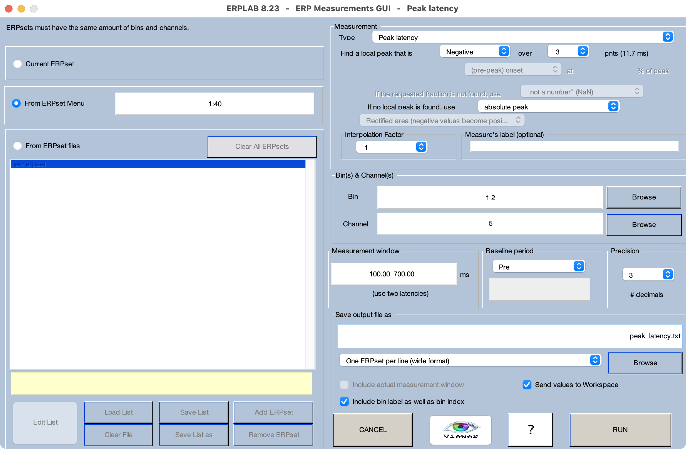
In the present exercise, we’re going to ask whether the peak latency of the LRP in the contralateral-minus-ipsilateral difference wave is later on incompatible trials than on compatible trials. Make sure that the 40 ERPsets from the previous exercise (from the Chapter_10 > Data > ERPsets_CI_Diff folder) are loaded. Launch the Measurement Tool and set it up as shown in Screenshot 10.5. The measurement Type is Peak latency, and we’re looking for a negative peak. We’re measuring from Bins 1 and 2 (Compatible and Incompatible) in the C3/C4 channel, and we’re saving the scores in a file named peak_latency.txt.
A key question in scoring ERP amplitudes and latencies is how to determine the time window. This is a complicated question, and you can read about several strategies in Chapter 9 of Luck (2014) and in Luck and Gaspelin (2017). As mentioned earlier, the most important thing is to avoid being biased by the data, which is best achieved by deciding on the measurement windows before you start the study. Of course, it’s too late for that now with the ERP CORE experiments. However, if I were to choose a time window in advance for the LRP in a flankers paradigm, I’d assume that the LRP begins after 100 ms and ends by 700 ms. For this reason, we’ll use a measurement window of 100 to 700 ms in this exercise.
Screenshot 10.5
As always, the next step is to click the Viewer button to see how well the algorithm is working. You’ll see that it has mixed success. It works reasonably well for waveforms that are clean and contain a large peak (e.g., File 2), but the scores are distorted by high-frequency noise (e.g., Files 1 and 12), and the values are largely random for waveforms without a distinct peak (e.g., Files 9 and 10).
Now go back to the Measurement Tool and click RUN to save the scores. Load the data into your statistics package and perform a paired t test to compare the Compatible and Incompatible conditions. Verify that the means provided by the statistics package are reasonable. You should see a mean of 318 ms for Compatible and 375 ms for Incompatible. Unfortunately, the trick we used with mean amplitude—comparing the means from the statistical package with the values measured from the grand average—doesn’t work with peak latency. If you measure the peak latency directly from the grand average ERP waveforms, you’ll see a value of 285 ms for Compatible and 355 ms for Incompatible. The values from the grand average aren’t the same as the mean of the single-subject values, but at least they show the same ordering (Compatible < Incompatible).
Now look at the actual t test results. You should see that the peak latency was significantly shorter for Compatible trials than for Incompatible trials (t(39) = -3.647, p < .001). Given the huge differences between Compatible and Incompatible trials in the grand average waveforms (Figure 10.2.C), it’s not surprising that the difference in peak latency was significant, even if peak latency isn’t an ideal scoring algorithm. You should also look at the effect size, measured as Cohen’s dz, which indicates how far apart the means are relative to the pooled standard deviation. You should see an effect size of -0.577 (or +0.577, depending on the order of conditions in your analysis), which is a medium effect size.
If you’re familiar with effect sizes in ERP studies, you might be surprised that this effect size isn’t bigger. After all, the peaks in the grand averages are very far apart in time. It therefore seems reasonable to suppose that we had a lot of measurement error when we computed the peak latency, which increased the standard deviation of the scores and therefore reduced the effect size. Given that peak latency scores are distorted by high-frequency noise, we should be able to reduce the measurement error and increase the effect size by applying a low-pass filter to the averaged ERPs prior to obtaining the peak latency scores.
Let’s try it. It would take quite a while for you to filter all 40 of the ERPsets using the GUI, so I’ve provided the ERPsets for you in Chapter_10 > Data > ERPsets_CI_Diff_filt. They’ve been low-pass filtered with a half-amplitude cutoff of 20 Hz and a slope of 12 dB/octave. Clear out the existing ERPsets from ERPLAB, load the filtered ERPsets, and repeat the measurement and analysis procedure (but changing the name of the measurement file to peak_latency_filt.txt). You’ll see that the effect size is now a little larger (d = -0.630). So, filtering helped, but only a little. Sometimes it helps a lot, especially when there is a lot of high-frequency noise in the data (which is not true for most of the waveforms in this experiment).