4.5: The Connectionist Sandwich
- Page ID
- 21225
Both the McCulloch-Pitts neuron (McCulloch & Pitts, 1943) and the perceptron (Rosenblatt, 1958, 1962) used the Heaviside step function to implement the all-ornone law. As a result, both of these architectures generated a “true” or “false” judgment about each input pattern. Thus both of these architectures are digital, and their basic function is pattern recognition or pattern classification.
The two-valued logic that was introduced in Chapter 2 can be cast in the context of such digital pattern recognition. In the two-valued logic, functions are computed over two input propositions, p and q, which themselves can either be true or false. As a result, there are only four possible combinations of p and q, which are given in the first two columns of Table 4-1. Logical functions in the two-valued logic are themselves judgments of true or false that depend on combinations of the truth values of the input propositions p and q. As a result, there are 16 different logical operations that can be defined in the two-valued logic; these were provided in Table 2-2.
The truth tables for two of the sixteen possible operations in the two-valued logic are provided in the last two columns of Table 4-1. One is the AND operation (p·q), which is only true when both propositions are true. The other is the XOR operation (p∧q), which is only true when one or the other of the propositions is true.
| p | q | p*q | p^q |
| 1 | 1 | 1 | 0 |
| 1 | 0 | 0 | 1 |
| 0 | 1 | 0 | 1 |
| 0 | 0 | 0 | 0 |
Table 4-1. Truth tables for the logical operations AND (p·q) and XOR (p ∧ q), where the truth value of each operation is given as a function of the truth of each of two propositions, p and q. ‘1’ indicates “true” and ‘0’ indicates “false.” The logical notation is taken from McCulloch (1988b).
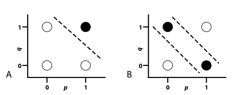
That AND or XOR are examples of digital pattern recognition can be made more explicit by representing their truth tables graphically as pattern spaces. In a pattern space, an entire row of a truth table is represented as a point on a graph. The coordinates of a point in a pattern space are determined by the truth values of the input propositions. The colour of the point represents the truth value of the operation computed over the inputs.
Figure 4-2A illustrates the pattern space for the AND operation of Table 4-1. Note that it has four graphed points, one for each row of the truth table. The coordinates of each graphed point—(1,1), (1,0), (0,1), and (0,0)—indicate the truth values of the propositions p and q. The AND operation is only true when both of these propositions are true. This is represented by colouring the point at coordinate (1,1) black. The other three points are coloured white, indicating that the logical operator returns a “false” value for each of them.

Figure 4-2. (A) Pattern space for AND; (B) Pattern space for XOR.
Pattern spaces are used for digital pattern recognition by carving them into decision regions. If a point that represents a pattern falls in one decision region, then it is classified in one way. If that point falls in a different decision region, then it is classified in a different way. Learning how to classify a set of patterns involves learning how to correctly carve the pattern space up into the desired decision regions.
The AND problem is an example of a linearly separable problem. This is because a single straight cut through the pattern space divides it into two decision regions that generate the correct pattern classifications. The dashed line in Figure 4-2A indicates the location of this straight cut for the AND problem. Note that the one “true” pattern falls on one side of this cut, and that the three “false” patterns fall on the other side of this cut.
Not all problems are linearly separable. A linearly nonseparable problem is one in which a single straight cut is not sufficient to separate all of the patterns of one type from all of the patterns of another type. An example of a linearly nonseparable problem is the XOR problem, whose pattern space is illustrated in Figure 4-2B. Note that the positions of the four patterns in Figure 4-2B are identical to the positions in Figure 4-2A, because both pattern spaces involve the same propositions. The only difference is the colouring of the points, indicating that XOR involves making a different judgment than AND. However, this difference between graphs is important, because now it is impossible to separate all of the black points from all of the white points with a single straight cut. Instead, two different cuts are required, as shown by the two dashed lines in Figure 4-2B. This means that XOR is not linearly separable.
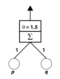
Linear separability defines the limits of what can be computed by a Rosenblatt perceptron (Rosenblatt, 1958, 1962) or by a McCulloch-Pitts neuron (McCulloch & Pitts, 1943). That is, if some pattern recognition problem is linearly separable, then either of these architectures is capable of representing a solution to that problem. For instance, because AND is linearly separable, it can be computed by a perceptron, such as the one illustrated in Figure 4-3.

Figure 4-3. A Rosenblatt perceptron that can compute the AND operation.
This perceptron consists of two input units whose activities respectively represent the state (i.e., either 0 or 1) of the propositions p and q. Each of these input units sends a signal through a connection to an output unit; the figure indicates that the weight of each connection is 1. The output unit performs two operations. First, it computes its net input by summing the two signals that it receives (the S component of the output unit). Second, it transforms the net input into activity by applying the Heaviside step function. The figure indicates in the second component of the output unit that the threshold for this activation function (q) is 1.5. This means that output unit activity will only be 1 if net input is greater than or equal to 1.5; otherwise, output unit activity will be equal to 0.
If one considers the four different combinations of input unit activities that would be presented to this device—(1,1), (1,0), (0,1), and (0,0)—then it is clear that the only time that output unit activity will equal 1 is when both input units are activated with 1 (i.e., when p and q are both true). This is because this situation will produce a net input of 2, which exceeds the threshold. In all other cases, the net input will either be 1 or 0, which will be less than the threshold, and which will therefore produce output unit activity of 0.
The ability of the Figure 4-3 perceptron to compute AND can be described in terms of the pattern space in Figure 4-2A. The threshold and the connection weights of the perceptron provide the location and orientation of the single straight cut that carves the pattern space into decision regions (the dashed line in Figure 4-2A). Activating the input units with some pattern presents a pattern space location to the perceptron. The perceptron examines this location to decide on which side of the cut the location lies, and responds accordingly.
This pattern space account of the Figure 4-3 perceptron also points to a limitation. When the Heaviside step function is used as an activation function, the perceptron only defines a single straight cut through the pattern space and therefore can only deal with linearly separable problems. A perceptron akin to the one illustrated in Figure 4-3 would not be able to compute XOR (Figure 4-2B) because the output unit is incapable of making the two required cuts in the pattern space.
How does one extend computational power beyond the perceptron? One approach is to add additional processing units, called hidden units, which are intermediaries between input and output units. Hidden units can detect additional features that transform the problem by increasing the dimensionality of the pattern space. As a result, the use of hidden units can convert a linearly nonseparable problem into a linearly separable one, permitting a single binary output unit to generate the correct responses.
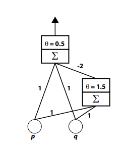
Figure 4-4 shows how the AND circuit illustrated in Figure 4-3 can be added as a hidden unit to create a multilayer perceptron that can compute the linearly nonseparable XOR operation (Rumelhart, Hinton, & Williams, 1986a). This perceptron also has two input units whose activities respectively represent the state of the propositions p and q. Each of these input units sends a signal through a connection to an output unit; the figure indicates that the weight of each connection is 1. The threshold of the output’s activation function (q) is 0.5. If we were to ignore the hidden unit in this network, the output unit would be computing OR, turning on when one or both of the input propositions are true.
However, this network does not compute OR, because the input units are also connected to a hidden unit, which in turn sends a third signal to be added into the output unit’s net input. The hidden unit is identical to the AND circuit from Figure 4-3. The signal that it sends to the output unit is strongly inhibitory; the weight of the connection between the two units is –2.

Figure 4-4. A multilayer perceptron that can compute XOR.
The action of the hidden unit is crucial to the behaviour of the system. When neither or only one of the input units activates, the hidden unit does not respond, so it sends a signal of 0 to the output unit. As a result, in these three situations the output unit turns on when either of the inputs is on (because the net input is over the threshold) and turns off when neither input unit is on. When both input units are on, they send an excitatory signal to the output unit. However, they also send a signal that turns on the hidden unit, causing it to send inhibition to the output unit. In this situation, the net input of the output unit is 1 + 1 – 2 = 0 which is below threshold, producing zero output unit activity. The entire circuit therefore performs the XOR operation.
The behaviour of the Figure 4-4 multilayer perceptron can also be related to the pattern space of Figure 4-2B. The lower cut in that pattern space is provided by the output unit. The upper cut in that pattern space is provided by the hidden unit. The coordination of the two units permits the circuit to solve this linearly nonseparable problem.
Interpreting networks in terms of the manner in which they carve a pattern space into decision regions suggests that learning can be described as determining where cuts in a pattern space should be made. Any hidden or output unit that uses a nonlinear, monotonic function like the Heaviside or the logistic can be viewed as making a single cut in a space. The position and orientation of this cut is determined by the weights of the connections feeding into the unit, as well as the threshold or bias (q) of the unit. A learning rule modifies all of these components. (The bias of a unit can be trained as if it were just another connection weight by assuming that it is the signal coming from a special, extra input unit that is always turned on [Dawson, 2004, 2005].)
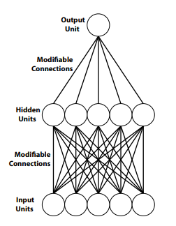
The multilayer network illustrated in Figure 4-4 is atypical because it directly connects input and output units. Most modern networks eliminate such direct connections by using at least one layer of hidden units to isolate the input units from the output units, as shown in Figure 4-5. In such a network, the hidden units can still be described as carving a pattern space, with point coordinates provided by the input units, into a decision region. However, because the output units do not have direct access to input signals, they do not carve the pattern space. Instead, they divide an alternate space, the hidden unit space, into decision regions. The hidden unit space is similar to the pattern space, with the exception that the coordinates of the points that are placed within it are provided by hidden unit activities.

Figure 4-5. A typical multilayer perceptron has no direct connections between input and output units.
When there are no direct connections between input and output units, the hidden units provide output units with an internal representation of input unit activity. Thus it is proper to describe a network like the one illustrated in Figure 4-5 as being just as representational (Horgan & Tienson, 1996) as a classical model. That connectionist representations can be described as a nonlinear transformation of the input unit representation, permitting higher-order nonlinear features to be detected, is why a network like the one in Figure 4-5 is far more powerful than one in which no hidden units appear (e.g., Figure 4-3).
When there are no direct connections between input and output units, the representations held by hidden units conform to the classical sandwich that characterized classical models (Hurley, 2001)—a connectionist sandwich (Calvo & Gomila, 2008, p. 5): “Cognitive sandwiches need not be Fodorian. A feed forward connectionist network conforms equally to the sandwich metaphor. The input layer is identified with a perception module, the output layer with an action one, and hidden space serves to identify metrically, in terms of the distance relations among patterns of activation, the structural relations that obtain among concepts. The hidden layer this time contains the meat of the connectionist sandwich.”
A difference between classical and connectionist cognitive science is not that the former is representational and the latter is not. Both are representational, but they disagree about the nature of mental representations. “The major lesson of neural network research, I believe, has been to thus expand our vision of the ways a physical system like the brain might encode and exploit information and knowledge” (Clark, 1997, p. 58).


