For readers who are interested in the sister subfield of bioarchaeology, which studies human remains and material culture from the past, please refer to chapter 8 of Bioarchaeology: Interpreting Human Behavior from Skeletal Remains, in TRACES: An Open Invitation to Archaeology (Blatt, Michael, and Bright forthcoming).
A forensic anthropologist should begin their analysis by reviewing the context in which the remains were discovered. This will help them understand a great deal about the remains, including determining whether they are archaeological or forensic in nature as well as considering legal and ethical issues associated with the collection, analysis, and storage of human remains (see “Ethics and Human Rights” section of this chapter for more information).
Figure 15.8: A human tooth with a filling. Credit: Filling by Kauzio has been designated to the public domain (CC0).
The “context” refers to the relationship the remains have to the immediate area in which they were found. This includes the specific place where the remains were found, the soil or other organic matter immediately surrounding the remains, and any other objects or artifacts in close proximity to the body. For example, imagine that a set of remains has been located during a house renovation. The remains are discovered below the foundation. Do the remains belong to a murder victim? Or was the house built on top of an ancient burial ground? Observing information from the surroundings can help determine whether the remains are archaeological or modern. How long ago was the foundation of the house erected? Are there artifacts in close proximity to the body, such as clothing or stone tools? These are questions about the surroundings that will help determine the relative age of the remains.
Clues directly from the skeleton may also indicate whether the remains are archaeological or modern. For example, tooth fillings can suggest that the individual was alive recently (Figure 15.8). In fact, filling material has changed over the decades, so the specific type of material used to fix a cavity can be matched with specific time periods. Gold was used in dental work in the past, but more recently composite (a mixture of plastic and fine glass) fillings have become more common.
How Many Individuals Are Present?
What Is MNI?
Another assessment that an anthropologist can perform is the calculation of the number of individuals in a mixed burial assemblage. Because not all burials consist of a single individual, it is important to burial assemblage be able to estimate the number of individuals in a forensic context. Quantification of the number of individuals in a burial assemblage can be done through the application of a number of methods, including the following: the Minimum Number of Individuals (MNI), the Most Likely Number of Individuals (MLNI), and the Lincoln Index (LI). The most commonly used method in biological anthropology, and the focus of this section, is determination of the MNI.
The MNI presents “the minimum estimate for the number of individuals that contributed to the sample” (Adams and Konigsberg 2008, 243). Many methods of calculating MNI were originally developed within the field of zooarchaeology for use on calculating the number of individuals in faunal or animal assemblages (Adams and Konigsberg 2008, 241). What MNI calculations provide is a lowest possible count for the total number of individuals contributing to a skeletal assemblage. Traditional methods of calculating MNI include separating a skeletal assemblage into categories according to the individual bone and the side the bone comes from and then taking the highest count per category and assigning that as the minimum number (Figure 15.9).
Figure 15.9: Skeletal elements from a commingled faunal assemblage. Credit: Commingled animal remains from Eden-Farson Pre-Contact site in southwest Wyoming by Matt O’Brien original to Explorations: An Open Invitation to Biological Anthropology (2nd ed.) is under a CC BY-NC 4.0 License.
Why Calculate MNI?
In a forensic context, the determination of MNI is most applicable in cases of mass graves, commingled burials, and mass fatality incidents. The term commingled is applied to any burial assemblage in which individual skeletons are not separated into separate burials. As an example, the authors of this chapter have observed commingling of remains resulting from mass fatality wildfire events. Commingled remains may also be encountered in events such as a plane or vehicle crash. It is important to remember that in any forensic context, MNI should be referenced and an MNI of one should be substantiated by the fact that there was no repetition of elements associated with the case.
Constructing the Biological Profile
Who Is It?
“Who is it?” is one of the first questions that law enforcement officers ask when they are faced with a set of skeletal remains. To answer this question, forensic anthropologists construct a biological profile (White and Folkens 2005, 405). A biological profile is an individual’s identifying characteristics, or biological information, which include the following: biological sex, age at death, stature, population affinity, skeletal variation, and evidence of trauma and pathology.
Forensic anthropologists typically construct a biological profile to help positively identify a deceased person. The following section will lay out each component of the biological profile and briefly review standard methodology used for each.
Assessing Biological Sex
Assessment of biological sex is often one of the first things considered when establishing a biological profile because several other parts, such as age and stature estimations, rely on an assessment of biological sex to make the calculations more accurate.
Assessment of biological sex focuses on differences in both morphological (form or structure) and metric (measured) traits in individuals. When assessing morphological traits, the skull and the pelvis are the most commonly referenced areas of the skeleton. These differences are related to sexual dimorphism usually varying in the amount of robusticity seen between males and females. Robusticity deals with strength and size; it is frequently used as a term to describe a large size or thickness. In general, males will show a greater degree of robusticity than females. For example, the length and width of the mastoid process, a bony projection located behind the opening for the ear, is typically larger in males. The mastoid process is an attachment point for muscles of the neck, and this bony projection tends to be wider and longer in males. In general, cranial features tend to be more robust in males (Figure 15.10).
When considering the pelvis, the features associated with the ability to give birth help distinguish females from males. During puberty, estrogen causes a widening of the female pelvis to allow for the passage of a baby. Several studies have identified specific features or bony landmarks associated with the widening of the hips, and this section will discuss one such method. The Phenice Method (Phenice 1969) is traditionally the most common reference used to assess morphological characteristics associated with sex. The Phenice Method specifically looks at the presence or absence of (1) a ventral arc, (2) the presence or absence of a subpubic concavity, and (3) the width of the medial aspect of the ischiopubic ramus (Figure 15.11). When present, the ventral arc, a ridge of bone located on the ventral surface of the pubic bone, is indicative of female remains. Likewise the presence of a subpubic concavity and a narrow medial aspect of the ischiopubic ramus is associated with a female sex estimation. Assessments of these features, as well as those of the skull (when both the pelvis and skull are present), are combined for an overall estimation of sex.
Metric analyses are also used in the estimation of sex. Measurements taken from every region of the body can contribute to estimating sex through statistical approaches that assign a predictive value of sex. These approaches can include multiple measurements from several skeletal elements in what is called multivariate (multiple variables) statistics. Other approaches consider a single measurement, such as the diameter of the head of the femur, of a specific element in a univariate (single variable) analysis (Berg 2017, 152–156).
It is important to note that, although forensic anthropologists usually begin assessment of biological profile with biological sex, there is one major instance in which this is not appropriate. The case of two individuals found in California, on July 8, 1979, is one example that demonstrates the effect age has on the estimation of sex. The identities of the two individuals were unknown; therefore, law enforcement sent them to a lab for identification. A skeletal analysis determined that the remains represented one adolescent male and one adolescent female, both younger than 18 years of age. This information did not match with any known missing children at the time.
In 2015, the cold case was reanalyzed, and DNA samples were extracted. The results indicated that the remains were actually those of two girls who went missing in 1978. The girls were 15 years old and 14 years old at the time of death. It is clear that the 1979 results were incorrect, but this mistake also provides the opportunity to discuss the limitations of assessing sex from a subadult skeleton.
Assessing sex from the human skeleton is based on biological and genetic traits associated with females and males. These traits are linked to differences in sexual dimorphism and reproductive characteristics between females and males. The link to reproductive characteristics means that most indicators of biological sex do not fully manifest in prepubescent individuals, making estimations of sex unreliable in younger individuals (SWGANTH 2010b). This was the case in the example of the 14-year-old girl. When examined in 1979, her remains were misidentified as male because she had not yet fully developed female pelvic traits.
Sex vs. Gender
Biological sex is a different concept than gender. While biological anthropologists can estimate sex from the skeleton, estimating an individual’s gender would require a greater context because gender is defined culturally rather than biologically. Take, for example, an individual who identifies as transgender. This individual has a gender identity that is different from their biological sex. The gender identity of any individual depends on factors related to self-identification, situation or context, and cultural factors. While in the U.S. we have historically thought of sex and gender as binary concepts (male or female), many cultures throughout the world recognize several possible gender identities. In this sense, gender is seen as a continuous or fluid variable rather than a fixed one.
Historically, forensic anthropologists have used a binary construct to categorize human skeletal remains as either male or female (with the accompanying categories of probable male, probable female, and indeterminate). In the case of transgender and gender nonconforming individuals, the binary approach to sex assessment may delay or hinder identification efforts (Buchanan 2014; Schall, Rogers, and Deschamps-Braly 2020; Tallman, Kincer, and Plemons 2021). As such, many forensic anthropologists have begun to address the inherent problems associated with a binary approach to sex identification and to explore ways of assessing social identity and self-identified gender using skeletal remains and forensic context.
For the duration of this section, the term transgender refers to individuals whose gender identity differs from the sex assigned at birth (Schall, Rogers, and Deschamps-Braly 2020:2). Transgender individuals transition from one gender binary to another, such as male-to-female (MTF) or female-to-male (FTM). While many of the gender-affirming procedures available to trans and gender-nonconforming individuals are focused on soft tissue modifications (e.g., breast augmentation, genital reconstruction, hormone therapies, etc.), there are a number of gender-affirmation surgeries that do leave a permanent record on the skeleton. Generally speaking, FTM transgender people are reported to undergo fewer surgical procedures than do MTF transgender people (Buchanan 2014). The discussion below focuses on Facial Feminization Surgery (FFS), which leaves a permanent record on the human skeleton that may be used to help make an identification.
FFS refers to a combination of procedures focused on sexually dimorphic features of the face, with the intent of transforming typically male facial features into more feminine forms. Facial Feminization Surgery procedures were developed by Dr. Douglas Ousterhout, a San Francisco based cranio-maxillofacial surgeon, in the mid-1980s (Schall, Rogers, and Deschamps-Braly 2020:2). FFS can include one or a combination of the following: hairline lowering, forehead reduction and contouring, brow lift, reduction rhinoplasty, cheek enhancement, lift lift, lip filling, chin contouring, jaw contouring, and/or tracheal shave (Buchanan 2014; Schall, Rogers, and Deschamps-Braly 2020:2). Of the procedures outlined previously, four are known to directly affect the facial skeleton: forehead contouring, rhinoplasty, chin contouring, and jaw contouring (Buchanan 2014; Schall, Rogers, and Deschamps-Braly 2020:2).
Because FFS procedures have been widely documented in the medical (and more recently the forensic anthropological) literature, there are a number of indicators that a forensic anthropologist can use to make more informed evaluations of gender, including evidence of bone remodeling in sexually dimorphic regions of the skull (e.g., forehead, chin, jawline), as well as the presence of plates, pins, or other surgical hardware that may be evidence of FFS (Buchanan 2014; Schall, Rogers, and Deschamps-Braly 2020; Tallman, Kincer, and Plemons 2021). Additionally, some forensic anthropologists suggest cautiously integrating contextual information from the scene, such as personal effects, material evidence, and recovery scene information, into their evaluation of an individual’s social identity (Beatrice and Soler 2016; Birkby, Fenton, and Anderson 2008; Soler and Beatrice 2018; Soler et al. 2019; Tallman, Kincer, and Plemons 2021; Winburn, Schoff, and Warren 2016). The ultimate goal of many skeletal analyses is to make a positive identification on a set of unidentified remains.
Assessment of Population Affinity
Population affinity is another component of the biological profile. We use the term population affinity to refer to the variation seen among modern populations—variation that is both genetic and environmentally driven. The word affinity refers to similarities or relationships between individuals. As forensic anthropologists, we compare an unknown individual to multiple reference groups and look for the degree of similarity in observable traits with those groups. As noted previously, population affinity can aid law enforcement in their identification of missing persons or unknown skeletal remains.
Within the field of anthropology, the estimation of population affinity has a contentious history, and early attempts at classification were largely based on the erroneous assumption that an individual’s phenotype (outward appearance) was correlated with their innate intelligence and abilities (see Chapter 13 for a more in-depth discussion of the history of the race concept). The use of the term race is deeply embedded in the social context of the United States. In any other organism/living thing, groups divided according to the biological race concept would be defined as a separate subspecies. The major issue with applying the biological race concept to humans is that there are not enough differences between any two populations to separate on a genetic basis. In other words, biological races do not exist in human populations. However, the concept of race has been perpetuated and upheld by sociocultural constructs of race.
The conundrum for forensic anthropologists is the fact that while races do not exist on a biological level, we still socially recognize and categorize individuals based on their phenotype. Clearly, our phenotype is an important factor in not only how we are viewed by others but also how we identify ourselves. It is also a commonly reported variable. Often labeled as “race,” we are asked to report how we self-identify on school applications, government identification, surveys, census reports, and so forth. It follows then that when a person is reported missing, the information commonly collected by law enforcement and sometimes entered into a missing person’s database includes their age, biological sex, stature, and “race.” Therefore, the more information a forensic anthropologist can provide regarding the individual’s physical characteristics, the more he or she can help to narrow the search.
As an exercise, create a list of all of the women you know who are between the ages of 18 and 24 and approximately 5’ 4” to 5’ 9” tall. You probably have several dozen people on the list. Now, consider how many females you know who are between the ages of 18 and 24, are approximately 5’ 4” to 5’ 9” tall, and are Vietnamese. Your list is going to be significantly shorter. That’s how missing persons searches go as well. The more information you can provide regarding a decedent’s phenotype, the fewer possible matches law enforcement are left to investigate. This is why population affinity has historically been included as a part of the biological profile.
In an effort to combat the erroneous assumptions tied to the race concept, forensic anthropologists have attempted to reframe this component of the biological profile. The term race is no longer used in casework and teaching. Historically, the word ancestry is and was deemed a more appropriate way to describe an individual’s phenotype. However, in more recent years, forensic anthropologists have begun using the term population affinity, recognizing that we are basing our analysis on the similarities we see based on the reference samples we have available (Winburn and Algee-Hewitt 2021). An important note here is that it is possible to hinder identifications and harm individuals when tools like estimations of population affinity are misapplied, misinterpreted, or misused. For this reason, the field of forensic anthropology has ongoing conversations about the appropriateness of this analysis in the biological profile (Bethard and DiGangi 2020; Stull et al. 2021).
Traditionally, population affinity was accomplished through a visual inspection of morphological variants of the skull (morphoscopics). These methods focused on elements of the facial skeleton, including the nose, eyes, and cheek bones. However, in an effort to reduce subjectivity, nonmetric cranial traits are now assessed within a statistical framework to help anthropologists better interpret their distribution among living populations (Hefner and Linde 2018). Based on the observable traits, a macromorphoscopic analysis will allow the practitioner to create a statistical prediction of geographic origin. In essence, forensic anthropologists are using human variation in the estimation of geographic origin, by referencing documented frequencies of nonmetric skeletal indicators or macromorphoscopic traits.
Population affinity is also assessed through metric analyses. The computer program Fordisc is an anthropological tool used to estimate different components of the biological profile, including ancestry, sex, and stature. When using Fordisc, skeletal measurements are input into the computer software, and the program employs multivariate statistical classification methods, including discriminant function analysis, to generate a statistical prediction for the geographic origin of unknown remains based on the comparison of the unknown to the reference samples in the software program. Fordisc also calculates the likelihood of the prediction being correct, as well as how typical the metric data is for the assigned group.
Estimating Age-at-Death
Estimating age-at-death from the skeleton relies on the measurement of two basic physiological processes: (1) growth and development and (2) degeneration (or aging). From fetal development on, our bones and teeth grow and change at a predictable rate. This provides for relatively accurate age estimates. After our bones and teeth cease to grow and develop, they begin to undergo structural changes, or degeneration, associated with aging. This does not happen at such predictable rates and, therefore, results in less accurate or larger age-range estimations.
During growth and development stages, two primary methods used for estimations of age of subadults (those under the age of 18) are epiphyseal union and dental development. Epiphyseal union (or epiphyseal fusion) refers to the appearance and closure of the epiphyseal plates between the primary centers of growth in a bone and the subsequent centers of growth (see Figure 15.7). Prior to complete union, the cartilaginous area between the primary and secondary centers of growth is also referred to as the growth plates (Schaefer, Black, and Scheuer 2009). Different areas of the skeleton have documented differences in the appearance and closure of epiphyses, making this a reliable method for aging subadult remains (SWGANTH 2013).
As an example of its utility in the identification process, epiphyseal development was used to identify two subadult victims of a fatal fire in Flint, Michigan, in February 2010. The remains represented two young girls, ages three and four. Due to the intensity of the fire, the subadult victims were differentiated from each other through the appearance of the patella, the kneecap. The patella is a bone that develops within the tendon of the quadriceps muscle at the knee joint. The patella begins to form around three to four years of age (Cunningham, Scheuer, and Black 2016, 407–409). In the example above, radiographs of the knees showed the presence of a patella in the four-year-old girl and the absence of a clearly discernible patella in the three-year-old.
Dental development begins during fetal stages of growth and continues until the complete formation and eruption of the adult third molars (if present). The first set of teeth to appear are called deciduous or baby teeth. Individuals develop a total of 20 deciduous teeth, including incisors, canines, and molars. These are generally replaced by adult dentition as an individual grows (Figure 15.12). A total of 32 teeth are represented in the adult dental arcade, including incisors, canines, premolars, and molars. When dental development is used for age estimations, researchers use both tooth-formation patterns and eruption schedules as determining evidence. For example, the crown of the tooth forms first followed by the formation of the tooth root. During development, an individual can exhibit a partially formed crown or a complete crown with a partially formed root. The teeth generally begin the eruption process once the crown of the tooth is complete. The developmental stages of dentition are one of the most reliable and consistent aging methods for subadults (Langley, Gooding, and Tersigni-Tarrant 2017, 176–177).
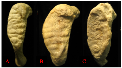
Degenerative changes in the skeleton typically begin after 18 years of age, with more prominent changes developing after an individual reaches middle adulthood (commonly defined as after 35 years of age in osteology). These changes are most easily seen around joint surfaces of the pelvis, the cranial vault, and the ribs. In this chapter, we focus on the pubic symphysis surfaces of the pelvis and the sternal ends of the ribs, which show metamorphic changes from young adulthood to older adulthood. The pubic symphysis is a joint that unites the left and right halves of the pelvis. The surface of the pubic symphysis changes during adulthood, beginning as a surface with pronounced ridges (called billowing) and flattening with a more distinct rim to the pubic symphysis as an individual ages. As with all metamorphic age changes, older adults tend to develop lipping around the joint surfaces as well as a breakdown of the joint surfaces. The most commonly used method for aging adult skeletons from the pubic symphysis is the Suchey-Brooks method (Brooks and Suchey 1990; Katz and Suchey 1986). This method divides the changes seen with the pubic symphysis into six phases based on macroscopic age-related changes to the surface. Figure 15.13 provides a visual of the degenerative changes that typically occur on the pubic symphysis.
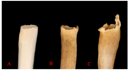
The sternal end of the ribs, the anterior end of the rib that connects via cartilage to the sternum, is also used in age estimations of adults. This method, first developed by M. Y. İşcan and colleagues, considers both the change in shape of the sternal end as well as the quality of the bone (İşcan, Loth, and Wright 1984; İşcan, Loth, and Wright 1985). The sternal end first develops a billowing appearance in young adulthood. The bone typically develops a wider and deeper cupped end as an individual ages. Older adults tend to exhibit bony extensions of the sternal end rim as attaching cartilage ossifies. Figure 15.14 provides a visual of the degenerative changes that typically occur in sternal rib ends.
Estimating Stature
Stature, or height, is one of the most prominently recorded components of the biological profile. Our height is recorded from infancy through adulthood. Doctor’s appointments, driver’s license applications, and sports rosters all typically involve a measure of stature for an individual. As such, it is also a component of the biological profile nearly every individual will have on record. Bioarchaeologists and forensic anthropologists use stature estimation methods to provide a range within which an individual’s biological height would fall. Biological height is a person’s true anatomical height. However, the range created through these estimations is often compared to reported stature, which is typically self-reported and based on an approximation of an individual’s true height (Ousley 1995).
In June 2015, two men were shot and killed in Granite Bay, California, in a double homicide. Investigators were able to locate surveillance camera footage from a gas station where the two victims were spotted in a car with another individual believed to be the perpetrator in the case. The suspect, sitting behind the victims in the car, hung his right arm out of the window as the car drove away. The search for the perpetrator was eventually narrowed down to two suspects. One suspect was 5’ 8” while the other suspect was 6’ 4”, representing almost a foot difference in height reported stature between the two. Forensic anthropologists were given the dimensions of the car (for proportionality of the arm) and were asked to calculate the stature of the suspect in the car from measurements of the suspect’s forearm hanging from the window. Approximate lengths of the bones of the forearm were established from the video footage and used to create a predicted stature range. Stature estimations from skeletal remains typically look at the correlation between the measurements of any individual bone and the overall measurement of body height. In the case above, the length of the right forearm pointed to the taller of the two suspects who was subsequently arrested for the homicide.
Certain bones, such as the long bones of the leg, contribute more to our overall height than others and can be used with mathematical equations known as regression equations. Regression methods examine the relationship between variables such as height and bone length and use the correlation between the variables to create a prediction interval (or range) for estimated stature. This method for calculating stature is the most commonly used method (SWGANTH 2012). Figure 15.15 shows the measurement of the bicondylar length of the femur for stature estimations.
Identification Using Individualizing Characteristics
One of the most frequently requested analyses within the forensic anthropology laboratory is assistance with the identification of unidentified remains. While all components of a biological profile, as discussed above, can assist law enforcement officers and medical examiners to narrow down the list of potential identifications, a biological profile will not lead to a positive identification. The term positive identification refers to a scientifically validated method of identifying previously unidentified remains. Presumptive identifications, however, are not scientifically validated; rather, they are based on circumstances or scene context. For example, if a decedent is found in a locked home with no evidence of forced entry but the body is no longer visually identifiable, it may be presumed that the remains belong to the homeowner. Hence, a presumptive identification.
The medicolegal system ultimately requires that a positive identification be made in such circumstances, and a presumptive identification is often a good way to narrow down the pool of possibilities. Biological profile information also assists with making a presumptive identification based on an individual’s phenotype in life (e.g., what they looked like). As an example, a forensic anthropologist may establish the following components of a biological profile: white male, between the ages of 35 and 50, approximately 5’ 7” to 5’ 11.” While this seems like a rather specific description of an individual, you can imagine that this description fits dozens, if not hundreds, of people in an urban area. Therefore, law enforcement can use the biological profile information to narrow their pool of possible identifications to include only white males who fit the age and height outlined above. Once a possible match is found, the decedent can be identified using a method of positive identification.
Positive identifications are based on what we refer to as individualizing traits or characteristics, which are traits that are unique at the individual level. For example, brown hair is not an individualizing trait as brown is the most common hair color in the U.S. But, a specific pattern of dental restorations or surgical implants can be individualizing, because it is unlikely that you will have an exact match on either of these traits when comparing two individuals.
A number of positive methods are available to forensic anthropologists, and for the remainder of this section we will discuss the following methods: comparative medical and dental radiography and identification of surgical implants.
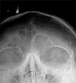
Comparative medical and dental radiography is used to find consistency of traits when comparing antemortem records (medical and dental records taken during life) with images taken postmortem (after death). Comparative medical radiography focuses primarily on features associated with the skeletal system, including trabecular pattern (internal structure of bone that is honeycomb in appearance), bone shape or cortical density (compact outer layer of bone), and evidence of past trauma, skeletal pathology, or skeletal anomalies. Other individualizing traits include the shape of various bones or their features, such as the frontal sinuses (Figure 15.16).
Comparative dental radiography focuses on the number, shape, location, and orientation of dentition and dental restorations in antemortem and postmortem images. While there is not a minimum number of matching traits that need to be identified for an identification to be made, the antemortem and postmortem records should have enough skeletal or dental consistencies to conclude that the records did in fact come from the same individual (SWGANTH 2010a). Consideration should also be given to population-level frequencies of specific skeletal and dental traits. If a trait is particularly common within a given population, it may not be a good trait to utilize for positive identification.
Surgical implants or devices can also be used for identification purposes (Figure 15.17). These implements are sometimes recovered with human remains. One of the ways forensic anthropologists can use surgical implants to assist in decedent identification is by providing a thorough analysis of the implant and noting any identifying information such as serial numbers, manufacturer symbols, and so forth. This information can then sometimes be tracked directly to the manufacturer or the place of surgical intervention, which may be used to identify unknown remains (SWGANTH 2010a).
Special Topic: Trans Doe Task Force
The Trans Doe Task Force (TDTF) is a Trans-led nonprofit organization that investigates cases involving LGBTQ+ missing and murdered persons. The organization specifically focuses on transgender and gender-variant cases, providing connections between law enforcement agencies, medical examiner offices, forensic anthropologists, and forensic genetic genealogists to increase the chances of identification. Additionally, the TDTF curates a data repository of missing, murdered, and unclaimed LGBTQ+ individuals, and they continuously try innovative approaches to identify these individuals, whose lived gender identity may not match their biological sex.