
5: Confidence Intervals
- Page ID
- 188424

\( \newcommand{\vecs}[1]{\overset { \scriptstyle \rightharpoonup} {\mathbf{#1}} } \)
\( \newcommand{\vecd}[1]{\overset{-\!-\!\rightharpoonup}{\vphantom{a}\smash {#1}}} \)
\( \newcommand{\id}{\mathrm{id}}\) \( \newcommand{\Span}{\mathrm{span}}\)
( \newcommand{\kernel}{\mathrm{null}\,}\) \( \newcommand{\range}{\mathrm{range}\,}\)
\( \newcommand{\RealPart}{\mathrm{Re}}\) \( \newcommand{\ImaginaryPart}{\mathrm{Im}}\)
\( \newcommand{\Argument}{\mathrm{Arg}}\) \( \newcommand{\norm}[1]{\| #1 \|}\)
\( \newcommand{\inner}[2]{\langle #1, #2 \rangle}\)
\( \newcommand{\Span}{\mathrm{span}}\)
\( \newcommand{\id}{\mathrm{id}}\)
\( \newcommand{\Span}{\mathrm{span}}\)
\( \newcommand{\kernel}{\mathrm{null}\,}\)
\( \newcommand{\range}{\mathrm{range}\,}\)
\( \newcommand{\RealPart}{\mathrm{Re}}\)
\( \newcommand{\ImaginaryPart}{\mathrm{Im}}\)
\( \newcommand{\Argument}{\mathrm{Arg}}\)
\( \newcommand{\norm}[1]{\| #1 \|}\)
\( \newcommand{\inner}[2]{\langle #1, #2 \rangle}\)
\( \newcommand{\Span}{\mathrm{span}}\) \( \newcommand{\AA}{\unicode[.8,0]{x212B}}\)
\( \newcommand{\vectorA}[1]{\vec{#1}} % arrow\)
\( \newcommand{\vectorAt}[1]{\vec{\text{#1}}} % arrow\)
\( \newcommand{\vectorB}[1]{\overset { \scriptstyle \rightharpoonup} {\mathbf{#1}} } \)
\( \newcommand{\vectorC}[1]{\textbf{#1}} \)
\( \newcommand{\vectorD}[1]{\overrightarrow{#1}} \)
\( \newcommand{\vectorDt}[1]{\overrightarrow{\text{#1}}} \)
\( \newcommand{\vectE}[1]{\overset{-\!-\!\rightharpoonup}{\vphantom{a}\smash{\mathbf {#1}}}} \)
\( \newcommand{\vecs}[1]{\overset { \scriptstyle \rightharpoonup} {\mathbf{#1}} } \)
\( \newcommand{\vecd}[1]{\overset{-\!-\!\rightharpoonup}{\vphantom{a}\smash {#1}}} \)
\(\newcommand{\avec}{\mathbf a}\) \(\newcommand{\bvec}{\mathbf b}\) \(\newcommand{\cvec}{\mathbf c}\) \(\newcommand{\dvec}{\mathbf d}\) \(\newcommand{\dtil}{\widetilde{\mathbf d}}\) \(\newcommand{\evec}{\mathbf e}\) \(\newcommand{\fvec}{\mathbf f}\) \(\newcommand{\nvec}{\mathbf n}\) \(\newcommand{\pvec}{\mathbf p}\) \(\newcommand{\qvec}{\mathbf q}\) \(\newcommand{\svec}{\mathbf s}\) \(\newcommand{\tvec}{\mathbf t}\) \(\newcommand{\uvec}{\mathbf u}\) \(\newcommand{\vvec}{\mathbf v}\) \(\newcommand{\wvec}{\mathbf w}\) \(\newcommand{\xvec}{\mathbf x}\) \(\newcommand{\yvec}{\mathbf y}\) \(\newcommand{\zvec}{\mathbf z}\) \(\newcommand{\rvec}{\mathbf r}\) \(\newcommand{\mvec}{\mathbf m}\) \(\newcommand{\zerovec}{\mathbf 0}\) \(\newcommand{\onevec}{\mathbf 1}\) \(\newcommand{\real}{\mathbb R}\) \(\newcommand{\twovec}[2]{\left[\begin{array}{r}#1 \\ #2 \end{array}\right]}\) \(\newcommand{\ctwovec}[2]{\left[\begin{array}{c}#1 \\ #2 \end{array}\right]}\) \(\newcommand{\threevec}[3]{\left[\begin{array}{r}#1 \\ #2 \\ #3 \end{array}\right]}\) \(\newcommand{\cthreevec}[3]{\left[\begin{array}{c}#1 \\ #2 \\ #3 \end{array}\right]}\) \(\newcommand{\fourvec}[4]{\left[\begin{array}{r}#1 \\ #2 \\ #3 \\ #4 \end{array}\right]}\) \(\newcommand{\cfourvec}[4]{\left[\begin{array}{c}#1 \\ #2 \\ #3 \\ #4 \end{array}\right]}\) \(\newcommand{\fivevec}[5]{\left[\begin{array}{r}#1 \\ #2 \\ #3 \\ #4 \\ #5 \\ \end{array}\right]}\) \(\newcommand{\cfivevec}[5]{\left[\begin{array}{c}#1 \\ #2 \\ #3 \\ #4 \\ #5 \\ \end{array}\right]}\) \(\newcommand{\mattwo}[4]{\left[\begin{array}{rr}#1 \amp #2 \\ #3 \amp #4 \\ \end{array}\right]}\) \(\newcommand{\laspan}[1]{\text{Span}\{#1\}}\) \(\newcommand{\bcal}{\cal B}\) \(\newcommand{\ccal}{\cal C}\) \(\newcommand{\scal}{\cal S}\) \(\newcommand{\wcal}{\cal W}\) \(\newcommand{\ecal}{\cal E}\) \(\newcommand{\coords}[2]{\left\{#1\right\}_{#2}}\) \(\newcommand{\gray}[1]{\color{gray}{#1}}\) \(\newcommand{\lgray}[1]{\color{lightgray}{#1}}\) \(\newcommand{\rank}{\operatorname{rank}}\) \(\newcommand{\row}{\text{Row}}\) \(\newcommand{\col}{\text{Col}}\) \(\renewcommand{\row}{\text{Row}}\) \(\newcommand{\nul}{\text{Nul}}\) \(\newcommand{\var}{\text{Var}}\) \(\newcommand{\corr}{\text{corr}}\) \(\newcommand{\len}[1]{\left|#1\right|}\) \(\newcommand{\bbar}{\overline{\bvec}}\) \(\newcommand{\bhat}{\widehat{\bvec}}\) \(\newcommand{\bperp}{\bvec^\perp}\) \(\newcommand{\xhat}{\widehat{\xvec}}\) \(\newcommand{\vhat}{\widehat{\vvec}}\) \(\newcommand{\uhat}{\widehat{\uvec}}\) \(\newcommand{\what}{\widehat{\wvec}}\) \(\newcommand{\Sighat}{\widehat{\Sigma}}\) \(\newcommand{\lt}{<}\) \(\newcommand{\gt}{>}\) \(\newcommand{\amp}{&}\) \(\definecolor{fillinmathshade}{gray}{0.9}\)This chapter is focused on confidence intervals. Next chapter we'll look at confidence intervals again, but with comparing subgroups.
We see polls in the news all the time, with claims about poll findings in headlines and media stories.
For example, when the Monmouth University Polling Institute released poll results, with this heading:
it generated news stories with headlines like the following:
"Poll: Support for NJ’s single-use plastic bag ban dips slightly" -NJBIZ
"Monmouth Poll: N.J. backs single-use plastic bag ban; oppose ban on paper bags at grocery stores" -New Jersey Globe
"Monmouth poll: One year later, New Jerseyans support plastic bag ban and have accumulated plenty of reusable bags" -ROI-NJ
"Poll: Support drops for NJ bag ban, 9% don't know it exists" -NJ 101.5
"New Poll Shows Majority of New Jersey Residents Oppose Ban on Grocery Paper Bags; Overall Support for Bag Ban Dips Slightly" -The Lakewood Scoop
What should we make of these headlines? Are they accurate? Do we need to be critical of such a poll?
The Monmouth University Polling Institute's findings are based on sample data. When they write in their release,
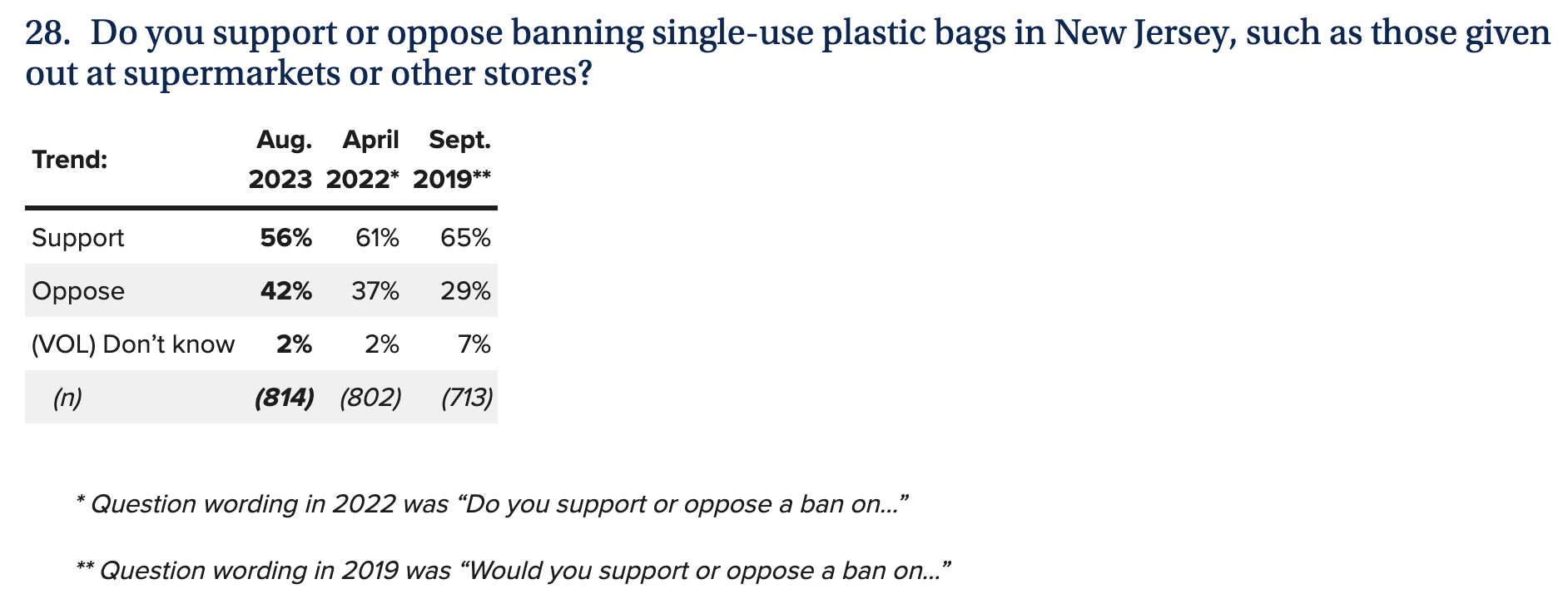
A majority of New Jerseyans continue to support a ban on single-use plastic bags (56%) although this is a few points lower than shortly before the ban went into effect (61% in April 2022).
they actually mean that 56% of 814 New Jersey adults they surveyed answered "support," when asked, "Do you support or oppose banning single-use plastic bags in New Jersey, such as those given out at supermarkets or other stores?"
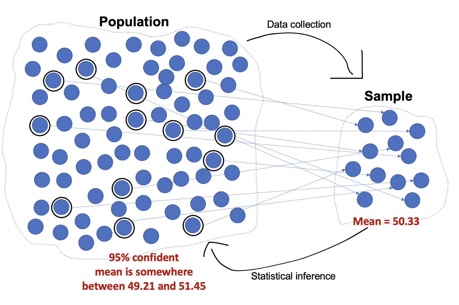
But nobody cares about what 814 random survey respondents think. We want to know about the target population, how New Jersey adults overall think. This is where we can turn to inferential statistics, and specifically confidence intervals.
Confidence Intervals
Confidence interval: The values within which we are claiming a population mean or proportion falls, at a particular confidence level, based on a representative sample of that population
As an example, in Chapter 3, I conducted a weighted analysis of an IPUMS dataset (IPUMS originally stood for Integrated Public Use Microdata Series) of American Community Survey (ACS) 5-Year Data for 2017 to 2021 and found that the sample mean annual income for full-time, year-round, non-institutionalized U.S. workers ages 16+ was $75,269.21.
At the 95% confidence level, the confidence interval for this mean is: $75,254.22, $75,284.21
The confidence interval consists of two numbers. I separate them with a comma because using a dash can be confusing (it also looks like a minus or negative sign).
The lower number, in this case $75,254.22, is called the lower limit or lower bound.
The greater number, in this case $75,284.21, is called the upper limit or upper bound.
We are 95% confident that the population mean is somewhere between the lower and upper bounds.
For a confidence interval of a mean:
General Template:
We are [confidence level, usually 95%] confident that, as of [date/time period sample data was collected], the mean [variable name/description] for [name of population] was somewhere between [lower limit with label] and [upper limit with label], meaning on average they were somewhere between [interpret lower limit and upper limit values in context].
Sometimes it flows better to name the population before the variable, e.g.,
[name of population]'s mean [variable name/description] (e..g, "U.S. adults' mean age" instead of "the mean age for U.S. adults").
Remember that to write the story of your confidence interval, you need to know information about your dataset (when was the data collected, who is the target population) and use your codebook to interpret the variable and values.
Note that the word "respondents" is not in the template. Respondents are those who responded to a survey --- they constitute the sample. Confidence intervals are about the target population.
Examples:
Previous chapters presented a number of sample means and proportions. Here are examples of interpreting some of their confidence intervals:
We can be 95% confident that, from 2017 to 2021, the mean income for full-time, year-round, civilian U.S. workers ages 16 or older was somewhere between $75,254.22 and $75,284.21. We are 95% confident that these workers average annual income was just over $75,000.
We are 95% confident that, from 2017 to 2021, the mean income for U.S. residents ages 16 or older was somewhere between $46,179.57 and $46,195.87. We are 95% confident that these residents average income was just over $46,000.
We are 95% confident that, following the 2020 general election, U.S. eligible voters mean feelings thermometer scores towards journalists were somewhere between 49.21 and 51.45, meaning on average they were neutral or close to neutral in their feelings towards journalists (the average is somewhere between just cooler or warmer than neutral).
Let's say there was a feelings thermometer questions about raspberries from the same dataset and we had a CI with a lower limit of 30 and upper limit of 70 (this is made up). In this case:
We are 95% confident that, following the 2020 general election, U.S. eligible voters mean feelings thermometer scores towards raspberries were somewhere between 30 and 70, meaning on average they were somewhere between fairly cold/unfavorable and fairly warm/favorable. We are fairly confident that on average they do not love or hate blueberries, but we're not really sure whether on average they feel more cold, neutral, or warm towards raspberries.
The confidence interval is providing a range within which we are confident (at 95% confidence, or whatever level specified) the population mean falls. It is only a claim about the population mean.
When we were dealing with sample data and normal distributions, we made estimates like "95% of data falls between ___ and ____." This is different than a confidence interval, which is based on a sampling distribution of means.
Take a look at a histogram of our sample ANES data about feelings towards journalists: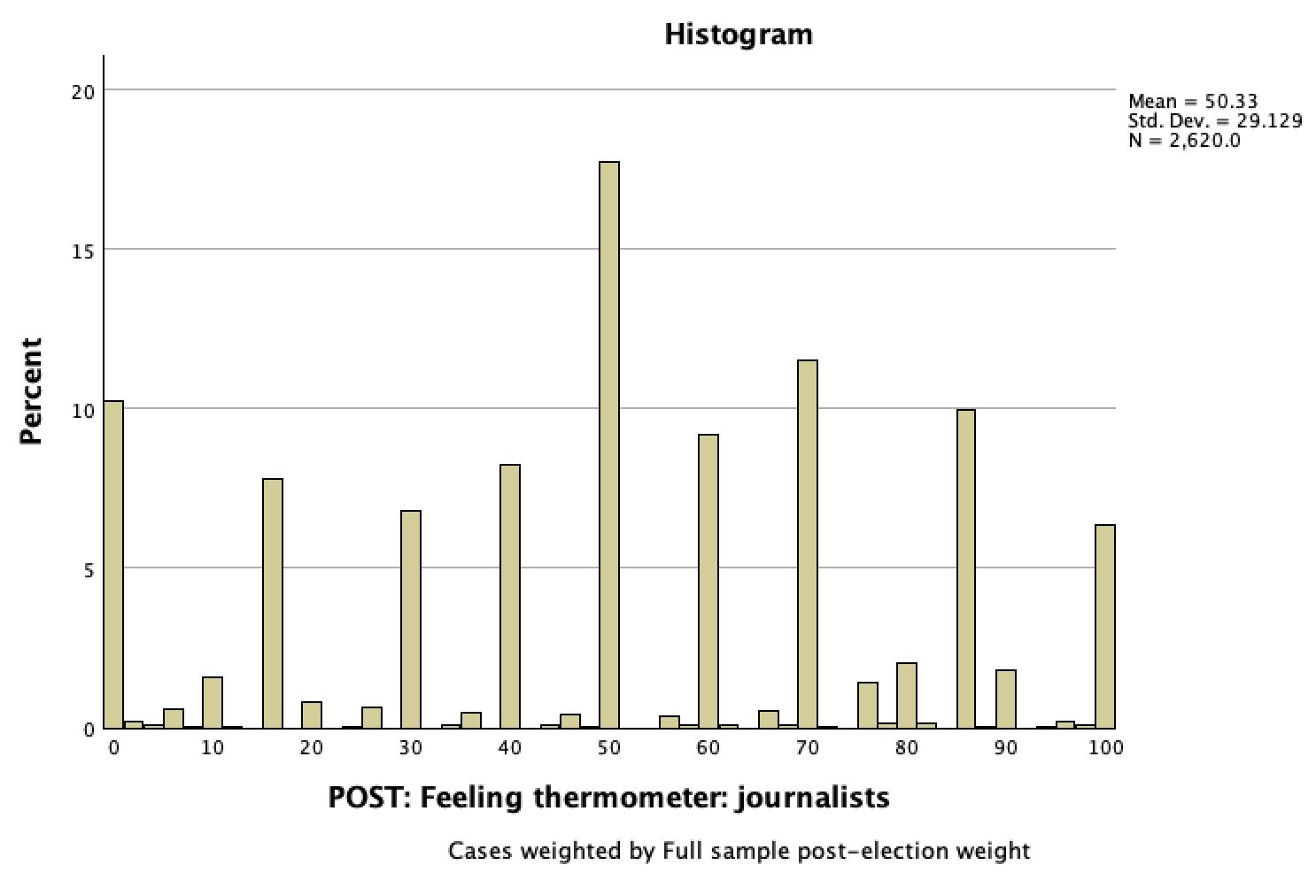
Our 95% CI is 49.21, 51.45.
It is wrong to interpret the CI by claiming that that 95% of respondents (or U.S. eligible voters) feelings thermometer scores were between 49.21 and 51.45 degrees. Take a look at the histogram --- within our sample, 95% of respondents were between 0 and 100 (there are over 2.5% of respondents at both 0 and 100). 95% of the respondents were not between 49.2 and 51.5 (less than 20% of respondents were), and it would not make sense that this would then be the case for all U.S. eligible voters.
Instead, take a look at the sample mean of 50.33. This is a sample mean. Due to sampling error, we're not confident this accurately reflects the population mean. So 50.33 is the mean for the 2,647 respondents in the sample, but we're not confident it would be the mean for all U.S. eligible voters. The 95% confidence interval is saying that we are 95% confident that the population mean is somewhere between 49.2 and 51.5. It cou50.33ld be 50.33, it could be 49.5, it could be 51.3, we're not sure. But based on the logic of sampling distributions and their properties, given that we have a probability sample, and given our sample mean, the sample size, and the level of variation in our data (as measured by standard deviation), we can make a claim at the 95% confidence level that the population mean is somewhere close to that sample mean, somewhere between 49.5 and 51.3. This is about the population mean, a measure of central tendency, not the distribution/spread of data/responses/feelings.
For a confidence interval of a proportion:
General Template:
We are [confidence level, usually 95%] confident that, as of [date/time period sample data was collected], somewhere between [lower limit] and [upper limit] of [name the population] [name the outcome].
For lower and upper limit, either use the percentages or convert these into benchmark fractions and say "about 1/5" or the like.
If you have already discussed when the sample was taken, you don't need to include its timing in your interpretation, but if this is new context, it's useful to know.
Example:
We are 95% confident that, as of 2022, somewhere between 36.7% and 39.9% (somewhere between 1/3 and 2/5) of U.S. adults have tried to encourage someone to believe in Jesus Christ or to accept Jesus Christ at their savior.
Note that the CI was: 0.367, 0.399. Because this was an indicator variable, I interpret these means as proportions (the percent with the value coded as 1).
For the Monmouth poll discussed above:
We are 95% confident that, in mid-August 2023, somewhere between 50.6% and 61.4% of New Jersey adults support banning single-use plastic bags in New Jersey, such as those given out at supermarkets or other stores.
Confidence intervals can be constructed at different confidence levels. The most widely used confidence level is 95%. If the confidence level is not specified, you can generally assume it is a 95% confidence interval. However, 90% confidence levels are also commonly used, such as by the U.S. Census.
What does it mean to say, "We are 95% confident?"
Confidence levels come from p-values (probability values).
A 95% confidence level is based on a p-value of 5%, or 0.05.
A 90% confidence level is based on a p-value of 10%, or 0.10.
To find your confidence level from a p-value, subtract it from 1 (or 100%). For example, for a p-value of 0.05 or 5%: 1-0.05=0.95 or 100%-5%=95%
The U.S. Census explains confidence intervals for a p-value of 5% this way:
If we were to repeatedly make new estimates using exactly the same procedure (by drawing a new sample, conducting new interviews, calculating new estimates and new confidence intervals), the confidence intervals would contain the average of all the estimates 95% of the time. We have therefore produced a single estimate in a way that, if repeated indefinitely, would result in 95% of the confidence intervals formed containing the true value.
Let's apply this using the confidence interval in the above example of feelings towards journalists. Consider what you know about sampling distributions and the Central Limit Theorem to make sense of this.
In the ANES survey following the 2020 general election, 2,647 U.S. eligible voters responded to a question about how they felt about journalists, and the sample mean was 50.33, a smidgen warmer than neutral.
Let's turn to the 95% confidence interval: 49.21, 51.45
If the population mean were actually less than 49.21 or more than 51.45, there is only a 5% chance ANES would have ended up drawing a random sample with the sample mean, sample size, and standard deviation of the variable in the sample. Given that ANES used probability sampling (generating a sample representative of their target population, though with sampling error), and given the ANES sample (the sample mean of 50.33, the sample size of 2,647, and the variability in the data with a standard deviation of 29.13), there is a 5% chance that the population mean is outside the parameters of our confidence interval (less than the lower bound of 49.21 or more than the upper bound of 51.45).
From this, we say we are 95% confident that the population mean is between 49.21 and 51.45.
ANES target population was all U.S. eligible voters. ANES collected data from a random sample of U.S. eligible voters. The sample mean was 50.33. While we know the sample mean, due to sampling error we're not sure about the population mean. However, we can be 95% confident it is somewhere between 49.21 and 51.45.
Population data:
Inferential statistics are not used with population data. Confidence intervals are not a relevant concept. If you have population data and have a mean, it's the population mean.
- The average age of a U.S. Senator (as of 2023) is 63.5 years old. This is based on a census of senators. There is no inference to make. We already know (with 100% confidence!) the population mean.
- In Chapter 1, 30% of the top 20 kids films between 2015 and August 2023 had monarchy as a central form of government (mean=0.15). We know the population mean/proportion and don't construct a confidence interval.
- In Chapter 3, you and your 9 friends each washed a mean of 5.5 cars. This was calculated based on a census of collecting data on every person who washed the cars and how many cars they washed. You would not construct a confidence interval. You already know the mean.
Non-representative samples:
- If you don't have a representative sample (based on probability sampling), you should not engage in inferential statistics.
- If you wanted to know what proportion of kids movies between 2015 and August 2023 had monarchy as a central form of government, you cannot figure this out using the sample of top 20 kids films. The top kids films may be different from all films, so it is not a representative sample.
- If you wanted to know how many cars people wash on average during a car wash, you cannot figure this out with your convenience sample of you and your friends. You and your friends may not be typical of car washers more broadly.
- If every person in the target population you want to generalize to did not have an equal chance of being selected to be part of the sample, inferential statistics are inappropriate.
You can use Explore/Examine in SPSS to construct confidence intervals.
Menu:
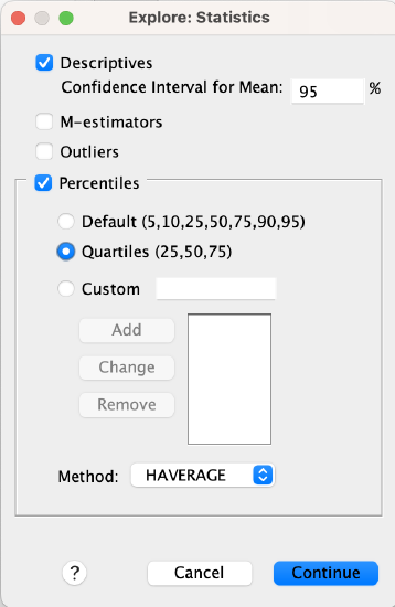
Go to Analyze → Descriptive Statistics → Explore. Put your variable into the Dependent List window/box. At the bottom where it says "Display," make sure you either have "Both" or "Statistics" checked (Plots will only give you graphs/figures).
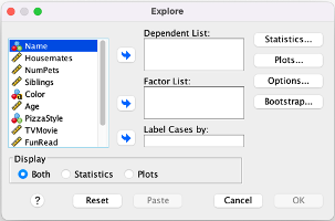
*If you want to construct a confidence interval at a confidence level other than 95%, click on the "Statistics" button, and where it says "Confidence Interval for Mean: 95%" replace the 95 with whatever confidence level you want to use.
Click OK to run the Explore command.
Syntax:
*This will generate a confidence interval along with other statistics.
EXAMINE VARIABLES=VariableName
/PLOT NONE
/PERCENTILES(25,50,75) HAVERAGE
/STATISTICS DESCRIPTIVES
/CINTERVAL 95
/MISSING LISTWISE
/NOTOTAL.
*If you want to construct a confidence interval at a confidence level other than 95%, replace the "95" on the /CINTERVAL line with the confidence level you want to use.
Reading the Output:
Here is what part of your output will look like:

In the Statistic column, the first row, "Mean," is your sample mean. The next two rows, "95% Confidence Interval for Mean," include your lower and upper bound for your confidence interval.
Remember that you can use this for proportions as well as long as your variable is set up as an indicator variable (dichotomous and coded 0 and 1).
If you are using population data, the first row (mean) is your population mean, and you would ignore the confidence interval rows.
You can generate a confidence interval using SPSS, but where do the numbers come from?
Looking back, when data has a standard normal distribution, you can find where a certain percentage of the data falls as follows:
Sample mean ± distance from mean = range of values
where Distance = Z-score x Standard deviation
For example, if you wanted to know between what two values about the middle 95% of data falls and have a mean of 10 and a standard deviation of 3,
- You know 95% of the data falls between approximately two standard deviation away from the mean, z=-2 to z=2
- The distance away from the mean will be the z-score x standard deviation, so 2*3=6
- The range of values will be the 10-6 and 10+6, so between 4 to 16
Confidence intervals work the same way, but using a normally distributed sampling distribution.
Mean ± distance from mean = confidence interval or: Proportion ± distance from proportion = confidence interval
Distance = t-score x standard error
Let's say we want to calculate a confidence interval with the same summary statistics, a mean of 10 and a standard deviation of 3.
Our mean is 10. Let's figure out the distance.
T-scores are based on t-distributions. A t-score for 95% of the area under the curve will be different depending on the curve, which depends on the sample size.

As the sample size gets large enough, the t-distribution will be a standard normal distribution, a z-distribution, and the t-score will equal the z-score, for a 95% confidence interval, 1.96.
There are t-tables you can use to look up approximate t-scores based on your selected confidence level and sample size, but you can do this more easily and precisely by using a t-score calculator. There are plenty online, such as this one.
When you use the online calculator, put your sample size in to the box that says "degree of freedom." For significance level, put in the p-value. Remember this is 1 minus your confidence level, so for a confidence level of 95%, you would put in 0.05 (1-0.95=0.05). Click calculate. Use the two-tailed t-value.
Let's use a sample size of 100. That gives us a t-score of 1.98.
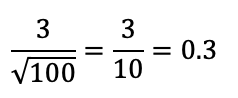
Standard Error, the standard deviation of the sampling distribution, is calculated based on the standard deviation and sample size.

In our case:
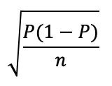
You can also calculate standard error for a proportion, using this formula:
Distance = t-score x standard error
Distance = 1.98 x 0.3 = 0.6
Mean ± distance from mean = confidence interval
10 ± 0.6 = confidence interval
10 - 0.6 = 9.4, our lower bound
10 + 0.6 = 10.6, our upper bound
Confidence interval (95% confidence level): 9.4, 10.6
Interpretation: I am 95% confident the population mean is somewhere between 9.4 and 10.6.
You will see polls in the news frequently. Oftentimes they have misleading headlines and text, where they report out sample poll data as if they are describing the population.
For example, in the Monmouth poll release, the article states:
Overall, 45% of New Jerseyans say, based on their own experience, all stores in the state are following the plastic bag ban and another 45% say most stores are.
However, 45% of New Jerseyans did not say this. 45% of the people who responded to their poll did.
Usually at the very end of articles you will find a mention of inferential statistics, but it is not incorporated into the article itself.
For example, in the Monmouth poll release, the last paragraph states:
The Monmouth University Poll was conducted by telephone from August 10 to 14, 2023 with 814 New Jersey adults. The question results in this release have a margin of error of +/- 5.4 percentage points for the full sample. The poll was conducted by the Monmouth University Polling Institute in West Long Branch, NJ.
When polls use the term margin of error (abbreviated as MOE), this is the same as distance from the mean/proportion that we were using above.
Oftentimes they give one margin of error, a "maximum margin of error," constructed based on a proportion of 50%. Margins of error would differ for more specific proportions.
To calculate a confidence interval, I would use the same formula.
So for example, for this question:
Confidence Interval = Sample mean/proportion ± margin of error
56% ± 5.4% would give me a 95% confidence interval of 50.6%, 61.4%
We are 95% confident that, in mid-August 2023, somewhere between 50.6% and 61.4% of New Jersey adults support banning single-use plastic bags in New Jersey, such as those given out at supermarkets or other stores.
While our confidence interval does indicate that, at 95% confidence level, a majority of New Jersey adults support the state's plastic bag ban, recall that the headline included a second claim: "Majority continues to back plastic bag ban, but at a slightly lower level."
Majority continues to back plastic bag ban, but at a slightly lower level. The provided sample statistics show that among those polled, support fell from 61% to 56% between April 2022 and August 2023. The April 2022 survey release indicated a margin of error of 3.5%. So, in April 2022, we can be 95% confident that somewhere between 57.5% and 64.5% of New Jersey adults supported the ban, and in August 2023, somewhere between 50.6% and 61.4% of New Jersey adults supported the ban. Yes, support could have fallen, but support could also be the same (it could have been 60% support both times), or it could have even increased (e.g., from 58% to 61%)! Be wary of discussions focused on changes in sample statistics that don't incorporate inferential statistics into their analyses. If I don't use the provided maximum margins of error and calculate my own for these proportions, I get 3.38% for 2022 and 3.42% for 2023. This makes the 95% confidence intervals for support 57.62% to 64.38% in 2022 and 52.58% to 59.42% in 2023. This still does not demonstrate, at 95% confidence, that there was a decrease in support.
Regardless, our confidence interval is only as good as our question and data. Notice that the Monmouth poll question forced people to choose if they supported or opposed the ban. No one was allowed to be neutral on it, unless they volunteered that they don't know, even though they weren't given that option as part of the question.
It's also critical to be careful about subgroups. Their given margin of error is for all 814 respondents. But if you get into questions about subgroups (e.g., particular age groups, genders, political parties, religions, etc.), this decreases the sample size and increases the margin of error.
Even when you account for sampling error, you still can't fix bad data. Be careful of non-scientific push polls that are used to get out certain message or to generate particular outcomes that can be promoted.
For example, take a look at this headline/release:
and this corresponding news story:

The reported margin of error is 3%, so with the survey findings that,
The latest Rasmussen Reports national telephone and online survey finds that 60% of Likely U.S. voters believe getting the migrant crisis at the U.S. border under control is more important for America’s national security, while 30% say supporting Ukraine in its war against Russia is more important. Another 10% are not sure.
we can be 95% confident that among U.S. likely voters, at least 23% more say migrant vs Ukraine.
But wait. Here are the first two survey questions:
1* Is the current situation with migrants at the U.S.-Mexico border a crisis?
2* Which is more important for America’s national security – getting the migrant crisis at the U.S. border under control, or supporting Ukraine in its war against Russia?
The survey wording labels one option as a crisis and portrays the Russia-Ukraine War as an act of aggression on Ukraine's part. Different survey wordings can lead to very different answers.
Confidence interval widths (the precision of your estimate) vary based on sample size, variation in sample data, and confidence levels.
Sample Size
- Larger samples have narrower confidence interval widths. You can make more precise predictions of the population mean.
- Smaller samples have wider confidence interval widths. With fewer cases, it's harder to be as sure about what the population mean is.
My university has about 13,000 students. If I were to randomly sample 100 students, it would be harder for me to make claims about the population with accuracy. If I were to randomly sample 1,000 students, I could do this with much more accuracy. If I were to randomly sample 12,000 students, my claims would be pretty precise.
Above, our confidence interval for the income of full-time, year-round, civilian U.S. workers ages 16. and older had a width of less than $30! A primary reason from this --- the sample had over 5 million cases! With that many randomly selected respondents from our target population, we can have much more certainty about the population mean.
Mathematically, a larger sample size will decrease the standard error and the t-score, which will make the distance/margin of error smaller.
That being said, at a certain point increasing the sample size does not affect the t-score much. At the 95% confidence level, a sample size of 120 has a t-score of 1.98, a sample size of 300 has a t-score of 1.97, a sample size of 500 has t-score of 1.96 (well, 1.96472), and a sample size of 1 million has a t-score of 1.96 (well, 1.959966). As the sample size increases, the t-distribution approaches a standard normal distribution, the z-distribution, and the t-score will equal the z-score.
Variation in Sample Data
- More variation (a larger standard deviation) widens confidence interval widths. With more uniformity, you can make more precise predictions of the population mean.
- Less variation (a smaller standard deviation) narrows confidence interval widths. With more variation, it's harder to be as sure what the population mean is.
If you randomly sample 200 people and they all have similar answers, you can be more comfortable estimating that the population mean is close to their mean. But if their answers have a lot of variation, there's more of a chance that sampling error might be impacting your mean.
Mathematically, more variation (a larger standard deviation) increases the standard error, which increases the distance/margin of error.
Confidence Levels
- Lower confidence levels (e.g., 80%) narrow confidence interval widths. If I don't have to be as confident the population mean is in my confidence interval, I can give a more precise estimate.
- Wider confidence levels (e.g., 99%) widen confidence interval widths. If I need to be more confident the population mean is in my confidence interval, I will give a broader range of possible means, increasing the chance the population mean is within that range.
Think about it. Using the feelings thermometer (0 cold to 100 warm) and a sample mean of 50, I can be 100% confident that a population mean will be somewhere between 0 and 100. I am not going to be as confident that the sample. mean is between 49.9 and 50.1.
You could make a really narrow confidence interval if you constructed a 50% or even 5% confidence interval. But this is useless. Who cares about your claim if you are only half confident or 5% confident that your population mean is within your interval. It's just as likely or more likely to be outside your interval!
Mathematically, higher confidence levels increase t-scores, which increases the distance/margin of error.