
7: Hypothesis Tests
- Page ID
- 188987

\( \newcommand{\vecs}[1]{\overset { \scriptstyle \rightharpoonup} {\mathbf{#1}} } \)
\( \newcommand{\vecd}[1]{\overset{-\!-\!\rightharpoonup}{\vphantom{a}\smash {#1}}} \)
\( \newcommand{\id}{\mathrm{id}}\) \( \newcommand{\Span}{\mathrm{span}}\)
( \newcommand{\kernel}{\mathrm{null}\,}\) \( \newcommand{\range}{\mathrm{range}\,}\)
\( \newcommand{\RealPart}{\mathrm{Re}}\) \( \newcommand{\ImaginaryPart}{\mathrm{Im}}\)
\( \newcommand{\Argument}{\mathrm{Arg}}\) \( \newcommand{\norm}[1]{\| #1 \|}\)
\( \newcommand{\inner}[2]{\langle #1, #2 \rangle}\)
\( \newcommand{\Span}{\mathrm{span}}\)
\( \newcommand{\id}{\mathrm{id}}\)
\( \newcommand{\Span}{\mathrm{span}}\)
\( \newcommand{\kernel}{\mathrm{null}\,}\)
\( \newcommand{\range}{\mathrm{range}\,}\)
\( \newcommand{\RealPart}{\mathrm{Re}}\)
\( \newcommand{\ImaginaryPart}{\mathrm{Im}}\)
\( \newcommand{\Argument}{\mathrm{Arg}}\)
\( \newcommand{\norm}[1]{\| #1 \|}\)
\( \newcommand{\inner}[2]{\langle #1, #2 \rangle}\)
\( \newcommand{\Span}{\mathrm{span}}\) \( \newcommand{\AA}{\unicode[.8,0]{x212B}}\)
\( \newcommand{\vectorA}[1]{\vec{#1}} % arrow\)
\( \newcommand{\vectorAt}[1]{\vec{\text{#1}}} % arrow\)
\( \newcommand{\vectorB}[1]{\overset { \scriptstyle \rightharpoonup} {\mathbf{#1}} } \)
\( \newcommand{\vectorC}[1]{\textbf{#1}} \)
\( \newcommand{\vectorD}[1]{\overrightarrow{#1}} \)
\( \newcommand{\vectorDt}[1]{\overrightarrow{\text{#1}}} \)
\( \newcommand{\vectE}[1]{\overset{-\!-\!\rightharpoonup}{\vphantom{a}\smash{\mathbf {#1}}}} \)
\( \newcommand{\vecs}[1]{\overset { \scriptstyle \rightharpoonup} {\mathbf{#1}} } \)
\( \newcommand{\vecd}[1]{\overset{-\!-\!\rightharpoonup}{\vphantom{a}\smash {#1}}} \)
\(\newcommand{\avec}{\mathbf a}\) \(\newcommand{\bvec}{\mathbf b}\) \(\newcommand{\cvec}{\mathbf c}\) \(\newcommand{\dvec}{\mathbf d}\) \(\newcommand{\dtil}{\widetilde{\mathbf d}}\) \(\newcommand{\evec}{\mathbf e}\) \(\newcommand{\fvec}{\mathbf f}\) \(\newcommand{\nvec}{\mathbf n}\) \(\newcommand{\pvec}{\mathbf p}\) \(\newcommand{\qvec}{\mathbf q}\) \(\newcommand{\svec}{\mathbf s}\) \(\newcommand{\tvec}{\mathbf t}\) \(\newcommand{\uvec}{\mathbf u}\) \(\newcommand{\vvec}{\mathbf v}\) \(\newcommand{\wvec}{\mathbf w}\) \(\newcommand{\xvec}{\mathbf x}\) \(\newcommand{\yvec}{\mathbf y}\) \(\newcommand{\zvec}{\mathbf z}\) \(\newcommand{\rvec}{\mathbf r}\) \(\newcommand{\mvec}{\mathbf m}\) \(\newcommand{\zerovec}{\mathbf 0}\) \(\newcommand{\onevec}{\mathbf 1}\) \(\newcommand{\real}{\mathbb R}\) \(\newcommand{\twovec}[2]{\left[\begin{array}{r}#1 \\ #2 \end{array}\right]}\) \(\newcommand{\ctwovec}[2]{\left[\begin{array}{c}#1 \\ #2 \end{array}\right]}\) \(\newcommand{\threevec}[3]{\left[\begin{array}{r}#1 \\ #2 \\ #3 \end{array}\right]}\) \(\newcommand{\cthreevec}[3]{\left[\begin{array}{c}#1 \\ #2 \\ #3 \end{array}\right]}\) \(\newcommand{\fourvec}[4]{\left[\begin{array}{r}#1 \\ #2 \\ #3 \\ #4 \end{array}\right]}\) \(\newcommand{\cfourvec}[4]{\left[\begin{array}{c}#1 \\ #2 \\ #3 \\ #4 \end{array}\right]}\) \(\newcommand{\fivevec}[5]{\left[\begin{array}{r}#1 \\ #2 \\ #3 \\ #4 \\ #5 \\ \end{array}\right]}\) \(\newcommand{\cfivevec}[5]{\left[\begin{array}{c}#1 \\ #2 \\ #3 \\ #4 \\ #5 \\ \end{array}\right]}\) \(\newcommand{\mattwo}[4]{\left[\begin{array}{rr}#1 \amp #2 \\ #3 \amp #4 \\ \end{array}\right]}\) \(\newcommand{\laspan}[1]{\text{Span}\{#1\}}\) \(\newcommand{\bcal}{\cal B}\) \(\newcommand{\ccal}{\cal C}\) \(\newcommand{\scal}{\cal S}\) \(\newcommand{\wcal}{\cal W}\) \(\newcommand{\ecal}{\cal E}\) \(\newcommand{\coords}[2]{\left\{#1\right\}_{#2}}\) \(\newcommand{\gray}[1]{\color{gray}{#1}}\) \(\newcommand{\lgray}[1]{\color{lightgray}{#1}}\) \(\newcommand{\rank}{\operatorname{rank}}\) \(\newcommand{\row}{\text{Row}}\) \(\newcommand{\col}{\text{Col}}\) \(\renewcommand{\row}{\text{Row}}\) \(\newcommand{\nul}{\text{Nul}}\) \(\newcommand{\var}{\text{Var}}\) \(\newcommand{\corr}{\text{corr}}\) \(\newcommand{\len}[1]{\left|#1\right|}\) \(\newcommand{\bbar}{\overline{\bvec}}\) \(\newcommand{\bhat}{\widehat{\bvec}}\) \(\newcommand{\bperp}{\bvec^\perp}\) \(\newcommand{\xhat}{\widehat{\xvec}}\) \(\newcommand{\vhat}{\widehat{\vvec}}\) \(\newcommand{\uhat}{\widehat{\uvec}}\) \(\newcommand{\what}{\widehat{\wvec}}\) \(\newcommand{\Sighat}{\widehat{\Sigma}}\) \(\newcommand{\lt}{<}\) \(\newcommand{\gt}{>}\) \(\newcommand{\amp}{&}\) \(\definecolor{fillinmathshade}{gray}{0.9}\)In the last chapter, we compared confidence intervals. This chapter will also involve inferential statistics that compare claims of population means, but through a slightly different approach: hypothesis testing. After reviewing one-sample t-tests, which are most similar to the logic of a confidence interval, we'll explore two-sample t-tests and one-way ANOVA. For these latter two tests, we'll also explore criteria for causality claims. These tests are about comparing means, so they will only work when your primary variable of interest is either ratio-like or an indicator variable.
1. Using a sample mean to judge the legitimacy of claims about a population: One-sample t-test
The General Social Survey, which is representative of U.S. adults, frequently includes the following survey question: "Tell me if you agree or disagree with this statement: Most men are better suited emotionally for politics than are most women."
Here are the historical results of the percentage that agreed:

Most recently, in 2022, 15.23% of respondents said they agree with the statement.
Less than one decade ago, this proportion was closer to 20%, or 1 in 5 respondents. Could it still be that 20% of U.S.-American adults would agree that women are generally less suitably emotionally for politics than men?
In Chapter 6, to answer this we would construct a 95% confidence interval to see if it does or does not overlap with 20%. If the confidence interval's upper bound was 20% or greater, that would mean that if the population proportion were really 20%, there is less than a 5% probability I would randomly draw this sample (given the sample proportion of 15.23% among 1,142 respondents).
Here is the confidence interval output from SPSS:
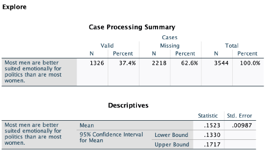
We are 95% confident that, as of 2022, somewhere between 13.3% and 17.2% of U.S. adults would agree that most men are better suited emotionally for politics than most women. This means we are also 95% confident that less than 20% of U.S. adults would agree.
While SPSS gives us a confidence interval, remember that behind the scenes it had to calculate the confidence interval bounds.
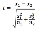
Here was our confidence interval formula:
T-score x Standard Error = Distance (or margin of error)
The t-score here assumes a 95% confidence level, which corresponds with that less than 5% probability that the population proportion is actually 20% (or any value outside the CI). This reflects back to sampling distributions and a normal t-distribution / bell curve, with the 5% on the tail ends. With a sample size over 1,000, our t-score for a 95% confidence level is 1.96.
SPSS gave us a standard error of 0.987%. We could calculate this as well, using the standard error formula for proportions or means: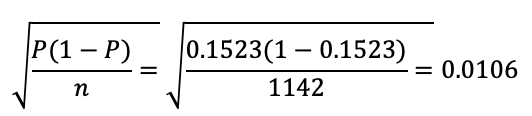
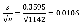
Both give me 0.987% (like SPSS) if I use the weighted sample size instead.
T-score x Standard Error = Distance (/Margin of Error)
1.96 x 0.00987 = 0.0193452 or 1.93%
15.23% + or - 1.93
CI: 13.30% to 17.16%
Okay, so we're over 95% confident that less than 20% of U.S. adults feel women are generally less suitably emotionally for politics than men. Are we over 99% confident?
I could answer this again by making another confidence interval:
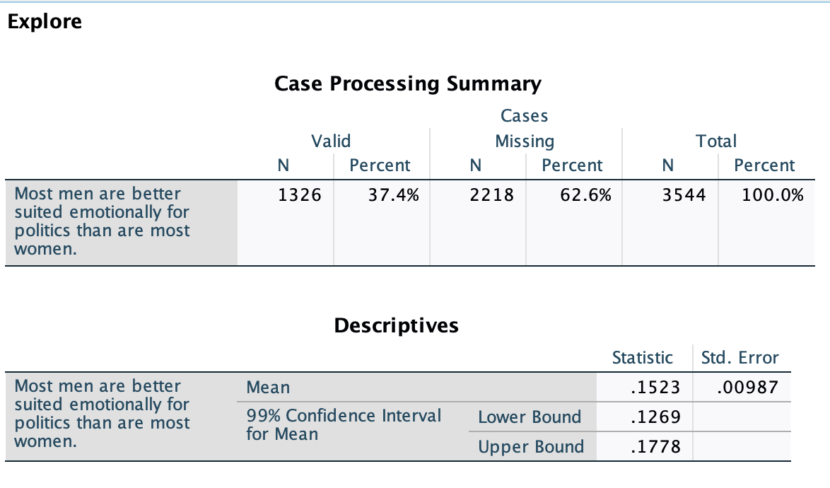
We are 99% confident that, as of 2022, somewhere between 12.7% and 17.8% of U.S. adults would agree that most men are better suited emotionally for politics than most women. This means we are also 99% confident that less than 20% of U.S. adults would agree.
Are we over 99.9% confident?
I could continue to test out different confidence intervals to find out how confident I can be. But there's another way to do this ---- called a one-sample t-test --- to find out how confident I can be that it's not actually 20% of U.S. adults that would agree that most men are better suited emotionally for politics than most women.
One-sample t-test: A statistical test used to evaluate claims about whether a population mean is different from a particular hypothesized value.
Do you remember fact families? For example, 2 groups of 3 will give me the same product as 3 groups of 2, 6. 6 divided into 2 groups gives me 3, and 6 divided into 2 groups will give me 3.

We can do the same thing with the confidence interval formula:
T-score x Standard Error = Distance
Distance / Standard Error = T-score
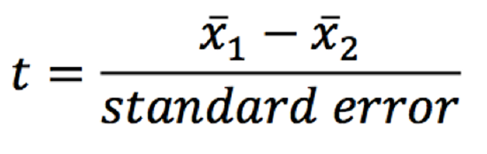
When we take the distance between two values, and divide them up by the standard deviation of the normal distribution, we can determine how many standard deviations/errors away the two values are from one another (our t-score). From there, we can figure out the probability and confidence level based on areas under the curve. For confidence intervals we had already put in a particular p-value (e.g., p=0.05) and corresponding confidence level (e.g., 95%), which we used along with sample size to determine the t-score, and eventually the distance. But if we already know distance, we can instead solve for the t-score, and then find out a particular probability and confidence level.
For a one-sample t-test, we want to figure out the probability that we would pull this random sample if the population proportion is actually 20% (or if the population mean is actually 0.2). We start with our distance (in this case the distance of the sample mean, 15.23%, from our test value for the population mean, in this case 20%) and use that and the standard error to calculate the t-score, and then from the t-score we can determine the p-value.
Let's try it:
Could the population mean be 20%
(If the population mean really were 20%, what is the probability that we would randomly pull this sample?)
Distance ÷ Standard Error = T-score
Distance = sample mean – test value = 15.23% – 20.00% = –4.77%
Standard Error = 0.00987 (calculated above)
Distance ÷ Standard Error = -4.77 ÷ 0.00987 = –483.28
The t-score, -483.28, represents how many standard errors 15.23% is away from 20.00%. We took the distance between the two means and made their units standard errors. This means that our sample mean is 483 standard errors less than / to the left of the test value of 20%.
You can use your t-score, with your sample size, to determine the p-value. Remember that different sample sizes determine what the normal t-distribution looks like and thus what the areas under the curve are. There are tables you can use to look up p-values based on a t-score and particular sample size, but instead we can just use an online calculator (such as this one), which will be easier and even more precise. If you use the linked online calculator, use the box "P from t", put the t-score in the box next to the t, and then where it says "DF," which stands for degrees of freedom, put in one less than the sample size. Click Compute P and we find that p<0.0001.
This means there is less than a 0.01% probability that we would randomly pull this sample if the population mean really where 20%.
To go from a p-value to a confidence level, 1-p, or if you have converted p into a percentage already, 100%-p%. For example, if p=0.05, 1-0.05=0.95 or 100%-5%=95%.
Here, p<0.0001, so 1-0.0001=0.9999, or 99.99%
We are over 99.99% confident that the population mean is not 20%.
That matches --- here's a confidence interval at the 99.99% confidence level. You can see the CI does not overlap 0.2:

You probably don't want to have to do those calculations each time. Here's how to conduct a one-sample t-test in SPSS:
SPSS: One-sample t-test
How to:
Menu option:
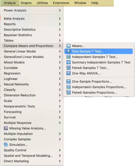
Analyze → Compare Means and Proportions → One-Sample T-test
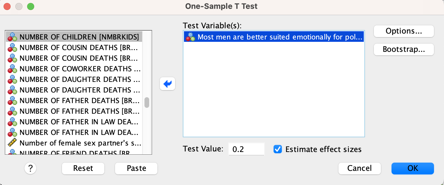
Select your variable. Write your hypothesized population mean in the test value box.
Syntax option:
T-TEST
/TESTVAL=TestValue#
/MISSING=ANALYSIS
/VARIABLES=VariableName
/CRITERIA=CI(.95).
Replace TestValue# with the test value (in this case 0.2) and VariableName with the name of your variable of interest.
Output:
Here is what your output will look like:
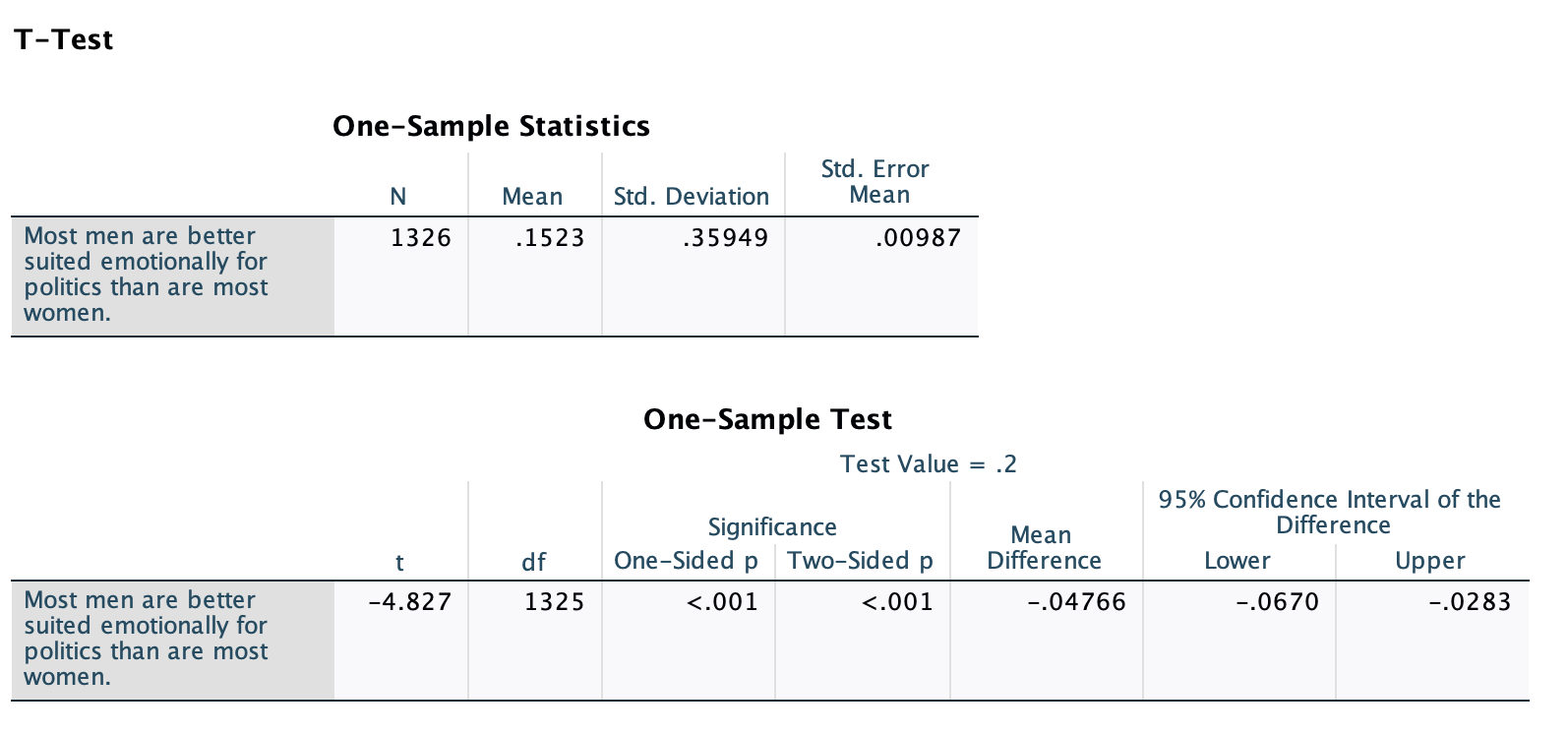
Here's how to interpret what's in the output:
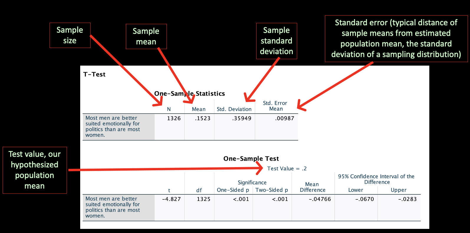
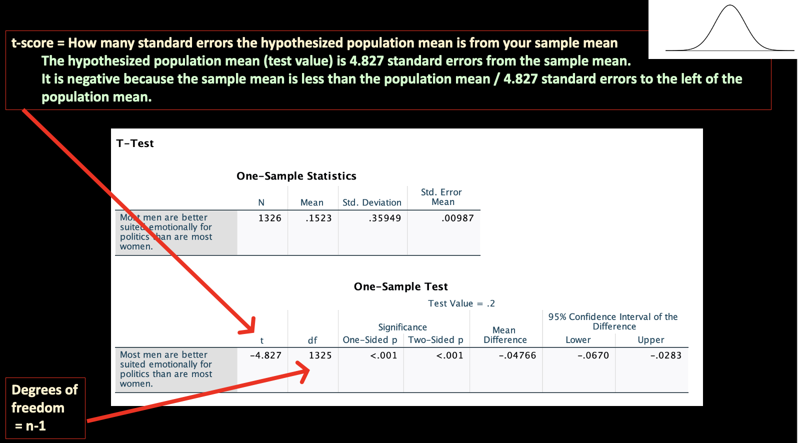 The more standard errors the sample mean and test population mean are from each other, the bigger the t-score.
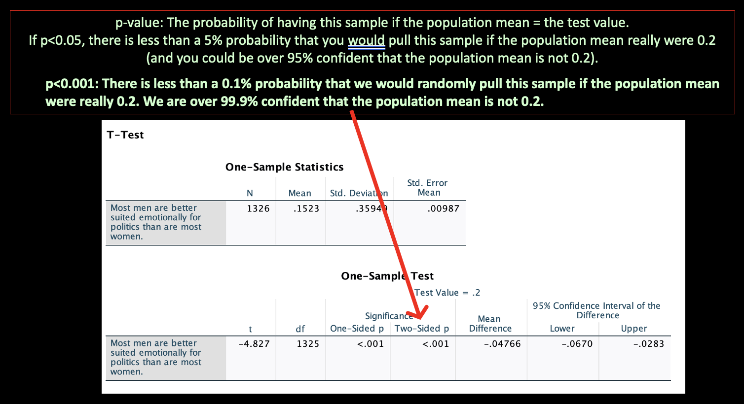
Use the "Two-sided p" under Significance. The one-sided p-value is based on a one-tailed test, which assumes a particular direction. If you think about the sampling distribution, the two-sided p reflects the area under the curve on both sides, at both tails.
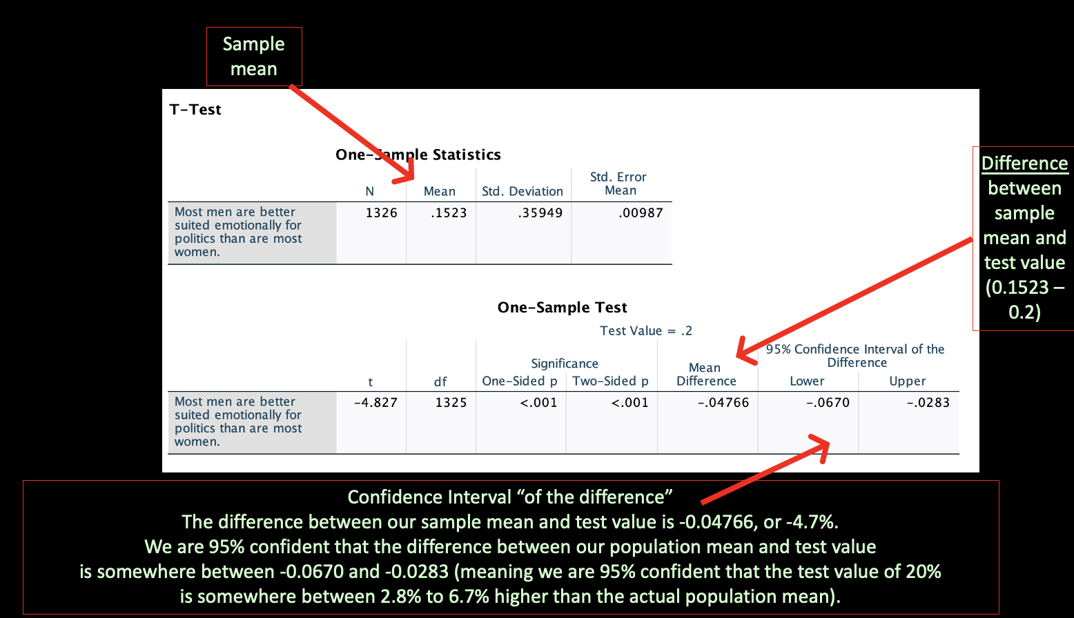
Don't get confused between "confidence intervals" like we covered in Chapters 5 and 6 and the "95% Confidence Interval of the Difference." Do you remember how we calculated how close and far apart two two population means or proportions might be from one another based on confidence intervals? This is more similar to those numbers. It's a confidence interval for how different the sample mean is from the test value. We know that the actual difference between our sample mean of 0.1523 and our test value of 0.2 is -0.04766. But due to sampling error, that might not be the actual difference among our target population. We are building a confidence interval around the difference between the two. If this confidence interval overlaps 0, then we know the population mean could be the test value (that they might be the same, at the 95% confidence level).
Hypothesis test (also known as "statistical test"): A statistical procedure that tests an inferential claim about a population using representative sample data.
We conduct “statistical tests” to test claims about a population based on sample data.
Hypothesis tests always start with a null and alternative hypothesis.
A hypothesis is a claim about a population based on statistics from a sample of this population. You can have your own hypotheses, but for statistical tests we will always have the same two:
H∅: Null hypothesis
The null hypothesis is always that there is no difference or no relationship (among your target population).
Ha: Alternative hypothesis
The alternative hypothesis is always that there is a difference or a relationship (among your target population).
Your statistical test will generate a "test statistic" (for one-sample t-tests, a t-value), which can be used to determine a p-value.
Conventionally, if p<0.05, you reject your null and accept your alternative hypothesis. This is a statistically "significant" difference or relationship. This means there is less than a 5% probability you would pull your sample if the null hypothesis were true.
Using p<0.05 as a cut-off point is arbitrary --- it's just based on convention. Why p<0.05 rather than p<0.01 or p<0.10, or something else? Does it really make sense to reject your null hypothesis if p=0.049 but fail to reject it if p=0.051? There are also different real-life situations where it might make more sense to lean towards having Type 1 errors (false positives, rejecting your null hypothesis when actually there is no difference/relationship) or Type 2 errors (false negatives, failing to reject your null hypothesis when actually there is a difference/relationship). Remember also that the probability-value is influenced by things like sample size. A p-value of <0.05 also does not tell you that a relationship matters or is important. A p-value is not a substitute for having to make judgments.
To this end, going forward I will be reporting out p<0.05 as significant, but also reporting out p<0.10 as marginally significant and p<0.15 as approaching significance, and using the following key to reflect various p-values:
^ p<0.15 ~ p<0.1 * p<0.05 ** p<0.01 *** p<0.001
Let's do a one-sample t-test, set up as a hypothesis test.
We are confident that it's not 20% (1/5) of U.S. adults who agree that "most men are better suited emotionally for politics than are most women." But could it be 1/6 (16.67%)? We already know that our 95% confidence interval overlapped 1/6, so we know p>0.05. We are not over 95% confident that the population mean is not 1/6. Let's find out what the probability is that we would pull this sample if the population proportion were actually 1/6.
Hypothesis Test
H∅: Null hypothesis: μ=16.67% (The population mean is 1/6)
(Our sample proportion was 15.23%. We're actually saying here that the sample mean of 15.23% could equal a population mean of 16.67%, that there's no significant difference.)
Ha: Alternative hypothesis: μ≠16.67% (The population mean is not 1/6)
(Our sample proportion was 15.23%. We're actually saying here that the sample mean of 15.23% does not equal a population mean of 16.67%, that there is a significant difference.)
One-sample t-test:

Test Statistic: t=-1.451 (Weighted) Sample size=1,326
P-value: 0.147 Confidence Level: 1-0.147=100%-14.7%=85.3%
Determination: Not significant (approaching significance)
Because p is not <0.05, we cannot reject our null or accept our alternative hypothesis. We are not over 95% confident that the population proportion is not 1/6. It could be. There is a 14.7% probability we would pull our sample if the population proportion were 1/6.
Notice how the 95% confidence interval of the difference overlaps 0. This means that we cannot be 95% confident that the population proportion is not the test value.
While not part of hypothesis tests, the next question we ask is whether there is substantive significance. Can we be 95% confident that there is a substantive or meaningful difference. Recall that we are 95% confident that, as of 2022, somewhere between 13.3% and 17.2% of U.S. adults would agree that most men are better suited emotionally for politics than most women. That's not substantively different from 16.67%, as it might be 16.67%. You could argue either way about whether it's substantively different from 20%. On the one hand, at the 95% confidence level, we're only confident that there's at least a 2.8% difference. On the other hand, that difference comes out to be over 9 million people, and elections can be pretty close.
You will not come across one-sample t-tests in sociology scholarship. One practical application for them would be if you have a variable about change that occurred and you want to compare that mean to a test value of zero to evaluate whether you can be confident there was any change. Regardless, let's move on to a statistical test you will see more often in the literature, the two-sample t-test.
2. Comparing two population means: two-sample t-test
While the one-sample t-test was more similar to in Chapter 5 when we constructed one confidence interval and saw what values were outside or inside its bounds, a two-sample t-test is somewhat similar to in Chapter 6 when we compared two confidence intervals to see whether or not they overlapped. Just like with the one-sample t-test, instead of starting with a confidence level and determining the distance, we'll start with a distance and determine the confidence level.
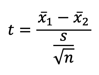
Remember that our formula for a one-sample t-test was:
t-score = distance ÷ standard error
It's the same for a two-sample t-test.
A t-score represents how many standard errors one population's mean is from the other. We take the distance and make its units standard errors, as reflected in this formula:
For a one-sample t-test:
Distance = sample mean – hypothesized population mean (test value)

For a two-sample t-test:
Distance = first sample mean – second sample mean

Rather than comparing a sample mean to a hypothesized population mean, we are comparing two sample means.
Rather than making an inference about the sample mean in terms of what population mean it could be and comparing that to a test value, we are making inferences about our sample means and comparing the two estimated population means.
Standard error has a similar formula, but it has to be modified because we now have two different samples, each with their own mean and standard error.
One-sample t-test: Two-sample t-test:
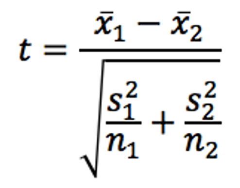
For the two-sample test, n1 is the sample size for the first group/subsample, and n2 is the sample size for the first group/subsample.
The further apart the two sample means are, the bigger the t-score.
The smaller the standard error, the bigger the t-score.
H∅: Null hypothesis: μ1=μ2
The null hypothesis is always that there is no difference or no relationship (among your target population).
Ha: Alternative hypothesis: μ1≠μ2 The population means are not equal.
The alternative hypothesis is always that there is a difference or a relationship (among your target population).
Your statistical test will generate a "test statistic" (for two-sample t-tests, a t-value), which can be used to determine a p-value.
Conventionally, if p<0.05, you reject your null and accept your alternative hypothesis. This is a statistically "significant" difference or relationship. This means there is less than a 5% probability you would pull your sample if the null hypothesis were true.
In Chapter 3 we looked at gender and race pay gaps. However, we were only looking at sample data. In this example we'll return to these pay gaps but evaluate them using statistical tests. Again, we're using 2017 to 2021 American Community Survey data. Our target population below will be full-time, year-round, non-institutionalized U.S. workers ages 16+.
A two-sample t-test only works for comparing two groups. In this case, we'll compare men and women's mean earnings.
H∅: Null hypothesis: μM=μW On average, men and women have the same incomes.
(There is no relationship between gender and income.)
Ha: Alternative hypothesis: μM≠μW On average, men and women have different incomes.
(There is a relationship between gender and income)
You might have your own hypothesis as well (e.g., men have higher average incomes than women), but our hypothesis test will only be evaluating the above.
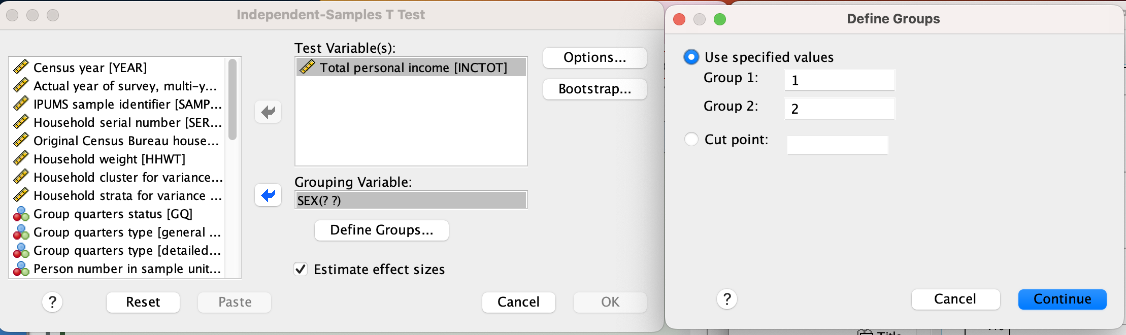
SPSS: Two-sample t-test
How to:
Menu option:
Analyze → Compare Means and Proportions → Independent-Samples T Test
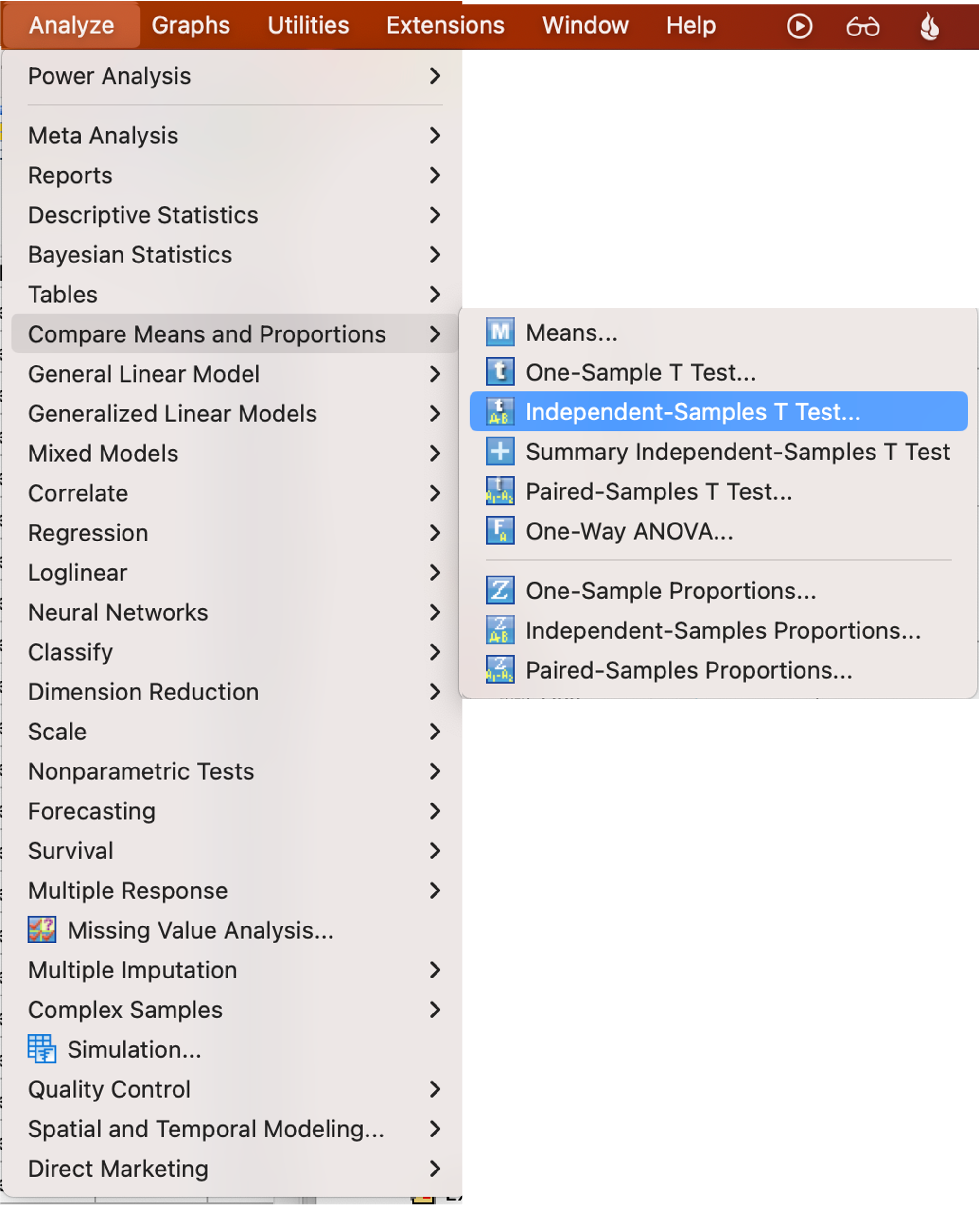
Select your test variable (the one you are interested in the means of, here the income variable).
Select your grouping variable (here gender).
Click "Define Groups" and then use the codes for the two groups you want to compare the means for. You have to look up the coding for the groups you have. Here it was 1 and 2. It could have been 0 and 8 or any other two numbers. You can do two-sample t-tests with a categorical variable that has more than two categories, as long as you only select two for comparison. After putting in your specified values, Click continue and then click OK.
Syntax option:
T-TEST GROUPS=GroupVariableName(# #)
/MISSING=ANALYSIS
/VARIABLES=TestVariableName
/CRITERIA=CI(.95).
Replace the #s with the codes for the categories you are using.
My syntax was:
T-TEST GROUPS=Sex(1 2)
/MISSING=ANALYSIS
/VARIABLES=IncTot
/CRITERIA=CI(.95).
Output:
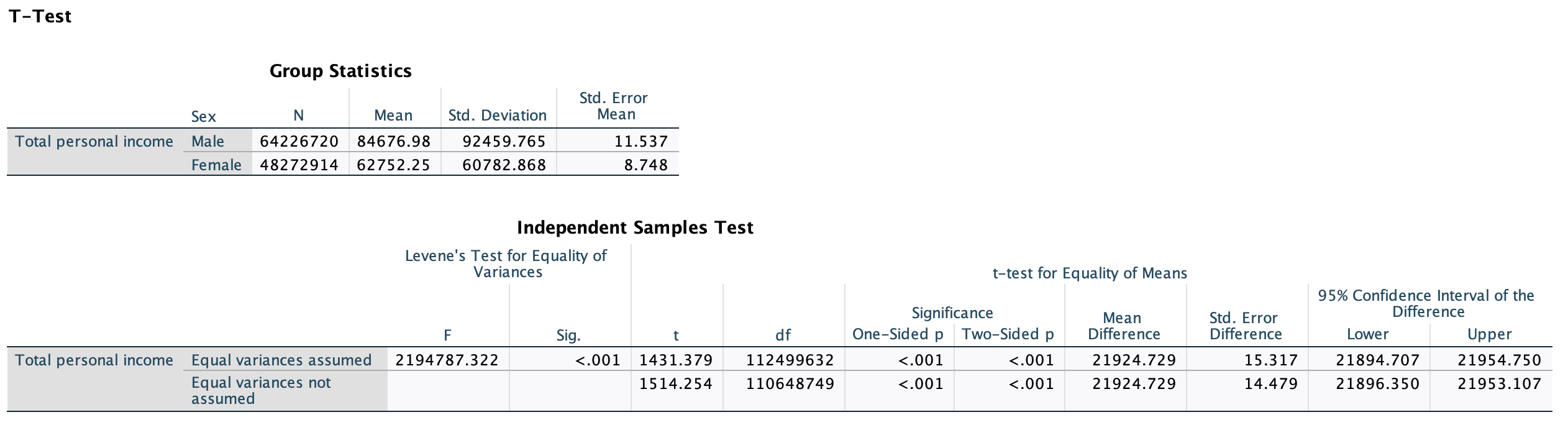
The descriptive statistics at the top shold look familiar to you. Now to the two-sample t-test. You have two different rows, but don't let that confuse you.
In order for statistical tests to work, there are a lot of assumptions that need to be met. For the two sample t-test, you either need samples of similar sizes or for the two samples to have equal variances. If you have similar sample sizes for the two groups or if the "Sig." p-value in the first row under "Levene's Test for Equality of Variances" is 0.05 or more, you can use the first row, the pooled two-sample t-test. If you do not have similar sample sizes for the two groups and the Sig. p-value under the Levene's test is <0.05, we need to use the second row, the unpooled two-sample t-test. The second row is more conservative as it is, and so if you'd prefer to just use that row to be on the safe side that is okay as well. The most important thing is to not confuse the Sig. in the second column, which is Levene's test, as being a p-value for the t-test, or to try to compare the first and second rows instead of just focusing on the row you are interpreting. If it's helpful, you can delete the first row (double-click on the output, highlight the first row, and right click and click delete).
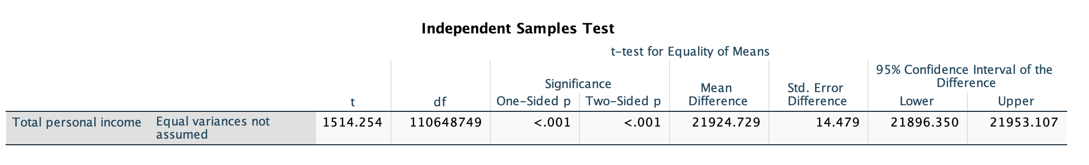 Let's take a look at this second row of the t-test. You'll see a t-score (1,514.254) and a p-value (use the "Two-sided p") of <0.001.
Because p<0.05, we can reject our null and accept our alternative hypothesis. There is less than a 0.1% probability that we would have pulled this sample if, between 2017 and 2021, men and women (who are full-time, year-round, non-institutionalized U.S. workers ages 16+) had the same mean earnings.
p<0.001 1-0.001=0.999=99.9% OR p<0.1% 100%-0.1%=99.9%
We are over 99.9% confident that men and women have different mean earnings.
(Note: I said over because p<0.001. If p=0.001 I would have said "We are 99.9% confident.")
All the way to the right you will notice a "95% Confidence Interval of the Difference." If this overlapped 0, we would know that men and women's mean earnings could be the same at the 95% confidence level.
Is it substantive?
Continuing to look at this output, the "mean difference" represents the first sample mean minus the second sample mean. Men's mean income was $84,676.98. Women's mean income was $62,752.25. The difference was $21,924.73. That's for the sample. Due to sampling error, we can only estimate how different men and women's mean incomes are. At the very right of the output we get a "95% Confidence Interval of the Difference." This is a confidence interval around the $21,924.73. We are 95% confident that, among our target population, men's mean income is somewhere between $21,953.11 and $21,896.35 more than women's mean income. Given that this is over $20,000, this definitely seems substantive.
Is it causal?
This is asking whether gender has an impact or effect on variation in income. I would argue it is causal. We have a significant and substantive relationship. The causal order makes sense: while gender might cause differences in pay, it would not make sense for how much one earns to change someone's gender. Gender is a relatively stable social location and patriarchy could impact the kinds of jobs and pay men vs. women earn. Theoretically, it makes sense that gender impacts mean earnings. There is a robust body of sociological scholarship expalining various reasons for the gender pay gap (e.g., the motherhood penalty and fatherhood bonus, pinkcollar jobs/workforce segregation and differential valuation, outright discrimination, etc.). There are no other preceding variables that would explain away this relationship.
Causality / Causation: There is a causal relationship when one variable has an impact or effect on variation of another variable.
When we are evaluating relationships between variables, we label one variable the "independent variable" (IV) and one variable the "dependent variable" (DV).
Dependent Variable: The outcome; the variable potentially being impacted by the independent variable
Independent Variable: The determinant; the variable potentially impacted the dependent variable
IV → DV
In the gender pay gap example, gender is the independent variable and income is the dependent variable. Gender is having an effect on income variation.
To determine causality, we need to conduct a controlled study and have validity and reliability. We can conduct an experiment and hold everything else constant other than the one thing we change, and simultaneously not change that factor for another group so we can make a comparison. But... human beings are not "guinea pigs." And we can't hold conditions constant while we conduct an experiment on ourselves. Also, these types of controlled studies would cost a ton of money. So, we do our best to make causal claims using the data and theory avialable to us.
There are five criteria that need to be met to claim causality. One can demonstrate causation is highly likely, but in social sciences it cannot be “proven.”
- Significance
- Substantiveness
- Correct causal order
- Theoretical sense/link/explanation
- Nonspuriousness
1. Significance
For a relationship to be causal, it must exist. Unless you are already looking at population data, this means that your inferential statistics test should show that the relationship is statistically significant. When we are testing for this relationship we are seeing whether the two variables co-vary, or vary together, also called covariance. This is often called association for qualitative measures and correlation for linear relationships.
2. Relationship is substantive
For us to claim that a relationship is causal, the relationship needs to be more than negligible. This may not be technically true --- if we had found that there was at least a $5 annual income mean difference between men and women, it could still be gender and patriarchy causing that difference --- but not enough for us to care. We want to look at relationships where the IV is having a substantial, meaningful imapct.
3. Causal order
We might have a significant and substantive relationship, but before we can claim the IV is impacting the DV, we have to make sure we correctly identified which variable is the IV and which is the DV. Does X cause Y or does Y cause X? Think about time order and what types of constructs are more stable. There are certain relationships that have a particular causal order and cannot be the other way around. For example, while race (through racism) can impact variation in birth weight, birth weight would not impact someone's racial classification. Or while region could have an impact on college graduation rates, college graduation rates are not going to impact geographic region.
4. Theory
The relationship has to have a sensical explanation. How does it make theoretical sense? We have to be able to provide a rationale for how the IV is impacting the DV.
5. Nonspuriousness
The relationship cannot be spurious. A spurious relationship is when a variable that precedes the IV explains away the entire relationship. While you can test this with multivariate analyses, this relies on theory to figure out what variables to test for (and you cannot test for it if you don't have the measures if your dataset). If a preceding variable only partially explains the relationship between the IV and DV, then the IV is still having its own causal impact, just a smaller one. We'll look at some examples of spurious relationships below, which will help make sense of this.
If there is a variable that comes after the first IV and before the second DV, it is okay for it to explain the relationship. This is not a challenge to the causality of the relationship. It is an explanation of how the IV impacts the DV, of its mechanism for doing so. For example, race impacts differentiation in political party registration. Obviously one’s race cannot automatically cause you to register with one party or the other. We can explain the relationship (social, economic, and racial equity policies of the two parties; racial representation in the parties; union relationships with the parties; parent/family/community political party allegiances, etc.) – but that is just explaining what makes it causal, not negating its causality.
There are lots of examples in the news, in social media, in politics, etc, where people claim causality when they shouldn't. Just because a relationship exists does not mean it is a causal relationship.
Consider the following existing relationships. What might be going on in these situations other than a causal relationship? Try to brainstorm your thoughts on each, then continue to scroll for the answers.
1. As the number of fire trucks sent to a fire increases, the amount of damage from the fire also increases. Does sending more fire trucks to a fire cause more damage to the place on fire?
2. Children who get tutored get worse grades than children who do not get tutored. Do children getting tutored cause them to get worse grades than children who do not get tutored?
3. When there are spikes in ice cream sales, there are also spikes in children drowning. Does ice cream cause kids to drown?
4. The more police in a community, the more crimes in said community. Does having more police in a community cause people to commit more crimes in that community?
6. On average, the bigger your palm, the shorter your lifespan. Does having a bigger palm cause you to have a shorter lifespan?
7. Do changes in the divorce rate in Maine cause U.S.-Americans to consume more/less margarine? They covary...
PAUSE HERE AND THINK THROUGH THE QUESTIONS ABOVE. WHEN YOU'RE READY, SCROLL DOWN FOR THE AnswerS.
Answers
Q1. As the number of fire trucks sent to a fire increases, the amount of damage from the fire also increases. Does sending more fire trucks to a fire cause more damage to the place on fire?
A1: This is a spurious relationship. The preceding variable is the size of the fire. Bigger fires lead to both more fire trucks being sent out and to fires that have more damage.
Q2. Children who get tutored get worse grades than children who do not get tutored. Do children getting tutored cause them to get worse grades than children who do not get tutored?
A2: The causal order is wrong. Children who are getting worse grades are more likely to seek out tutoring.
Q3. When there are spikes in ice cream sales, there are also spikes in children drowning. Does ice cream cause kids to drown?
A3: This is spurious. The preceding variable is weather. Hotter weather = more swimming (and thus more drowning) and more ice cream. Colder weather = less of both.
Q4. The greater the number of police in a community, the greater the number of crimes in said community. Does having more police in a community cause people to commit more crimes in that community?
A4: This is a spurious relationship. It's all about the population size of the community. There are going to be more police and more crimes in a community that has a million people vs. a community with 300 people.
Q5. Kids who sleep with the light on are more likely to become short-sighted adults. Does sleeping with the light on as a young kid is will cause you to be short-sighted later in life?
A5: This is spurious. Being short-sighted is genetic! So parents who are short-sighted are more likely to put on a night light and more likely to have short-sighted kids. The parents being or not being short-sighted is the preceding variable that explains away the relationship.
Q6. On average, the bigger your palm, the shorter your lifespan. Does having a bigger palm cause you to have a shorter lifespan?
A6: This is spurious. The preceding variables are sex and gender. Females on average have smaller palms than males, and females and women on average have longer lifespans than males and men.
Q7. Do changes in the divorce rate in Maine cause U.S.-Americans to consume more/less margarine? They covary...
A7: I have no explanation for this one. Strange things co-vary. If you look for patterns, you'll find them. You can find more of these at: http://www.tylervigen.com/spurious-correlations
There are usually multiple variables impacting a dependent variable. Just because other things also contribute, and maybe even more so then the independent variable you are looking at, does not mean you don't have a causal relationship. Causal just means the IV is impacted the DV, not that it is the only or main thing causing differentiation in the DV.
Example: Race, gender, and class all have causal impacts on who people vote for for president. There are many other things that influence who people vote for for president (e.g., political party, age, etc.). But none of these precede the other variables and explain away the entire relationship. While there are other determinants of who people vote, race, gender, and class still have a causal relationship with who people vote for.
3. Comparing more than two population means: one-way ANOVA
There are other types of t-tests besides one-sample and two-sample t-tests. For example, paired t-tests are used to compare before and after results. However, we're going to move to one final statistical test for this chapter, and it's not a t-test. Instead, let's turn to one-way ANOVA.
While a two-sample t-test allows us to evaluate, among our target population, whether the mean of a variable is different for two groups, what if you want to compare more than two groups?
There are various forms of ANOVA, but the one we're doing here, called a "one-way ANOVA," is for comparing means among more than two groups.
ANOVA stands for Analysis of Variance
ANOVA is similar to a two-sample t-test in that we are comparing means and then dividing it by a measure of variation for our samples.
two-sample t-test ANOVA
For ANOVA, we compare group means to the overall mean. If the group means are equal, they would each be the same as the population mean.
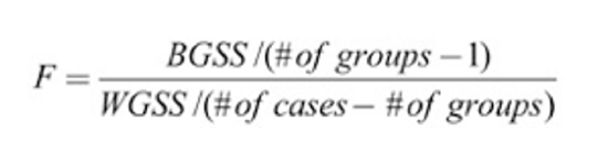
In the ANOVA equation above, BGGS stands for "Between Groups Sum of Squares." It is a measure of deviation between group means. The more deviation between group means, the bigger the BGSS, and the more likely to find that not all groups have the same means.
To calculate BGSS:
- Calculate the overall mean for all data
- Calculate the mean for each group
- For each group, find the difference between the group mean and the overall mean, and square it.
- For each group, multiply this by the number of cases (we are treating each case as if it had the group mean; we’ll account for within group variation later with WGSS)
- Add up these squared differences.
In the ANOVA equation above, WGSS stands for "Within Groups Sum of Squares." It is a measure of deviation within the groups. The more within group variation, the bigger the WGSS, and the less likely to find that not all groups have the same means.
Calculating ANOVA is very similar to calculating variance (which we do when we calculate standard deviation; variance is standard deviation squared). Here are the steps:
- For each group:
- Calculate the mean.
- Find the difference between each value and the mean.
- Square the differences.
- Add up the squared differences.
- Then add up each group's summed squared differences.
While confidence intervals and two-sample t-tests used normal t-distributions, ANOVA is different. It uses an F-distribution and the statistical test generates an F-statistic. F is the ratio of two variances (between group and within group). It is not a normal distribution (e.g., you can't have F=0 or F<0). While the t-distribution curves were based on sample size, the F-distribution is based both on sample size and on the number of groups you are comparing. However, it's otherwise the same idea. The area under the curve adds up to 1 (100%), the probability of observing any F value. The figure below shows various F-distribution curves. The legend shows "d" for degrees of freedom. These are based on number of groups and number of cases. Sometimes instead of seeing d1 and d2 or df1 and df2, you will see them referred to as the degrees of freedom for the numerator and denominator, because they are the formulas in parentheses in the F-statistic formula (df 1 = # of groups - 1; df2 = # of cases - # of groups).

•Once we have our F-value, we are going to have to use both the number of cases and number of groups to determine the right F-distribution. You can use the same webpage as for two-sample t-tests, but would fill out the P from F information. There it says DFn and DFd to refer to degrees of freedom from the numerator and degrees of freedom from the denominator.
H∅: Null hypothesis: μ1 = μ2 = μ3 … All the population means are equal
The null hypothesis is always that there is no difference or no relationship (among your target population).
Ha: Alternative hypothesis: The population means are not all equal. At least one population mean is different from at least one other population mean.
The alternative hypothesis is always that there is a difference or a relationship (among your target population).
Your statistical test will generate a "test statistic" (for one-way ANOVA, an F-statistic), which can be used to determine a p-value.
Conventionally, if p<0.05, you reject your null and accept your alternative hypothesis. This is a statistically "significant" difference or relationship. This means there is less than a 5% probability you would pull your sample if the null hypothesis were true.
If you reject your null hypothesis, you still do not know how many groups have different means, which groups are different, or the strength or direction of the difference.
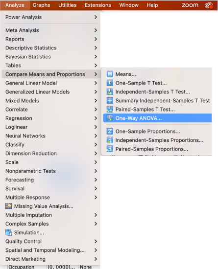
Menu option:
Analyze ➡ Compare Means and Proportions ➡ One-way ANOVA
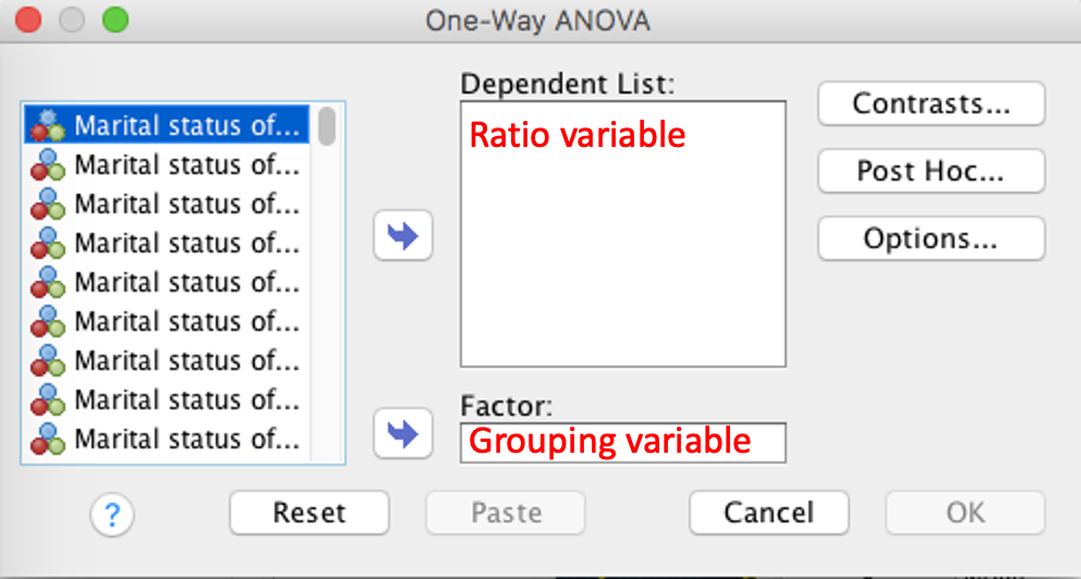
Put the variable you want means for in the dependent list box and the variable with your group categories in the factor box.
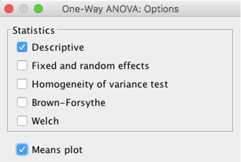
Click on Options and select Descriptive and Means plot.
Click Continue and then OK.
Syntax option:
ONEWAY RatioVariableName BY GroupingVariableName
/STATISTICS DESCRIPTIVES
/PLOT MEANS
/MISSING ANALYSIS.
Let's return to our 2017 to 2021 American Community Survey data. Our target population below will be full-time, year-round, non-institutionalized U.S. workers ages 16+. We're using ANOVA to compare average income by racial group because we have more than two racial groups. A two-sample t-test only works for comparing two groups. Because we want to compare more than two means, we're using ANOVA.
H∅: Null hypothesis: μW=μB=μA=μO=μH
On average, NH White, NH Black, NH API, NH Other/Multi, and Hispanic U.S. workers all have the same incomes.
(There is no relationship between race and income.)
Ha: Alternative hypothesis: Not all 5 racial groups have the same mean income. At least one racial group has a different mean income than at least one other racial group.
(There is a relationship between race and income)
SPSS Output:
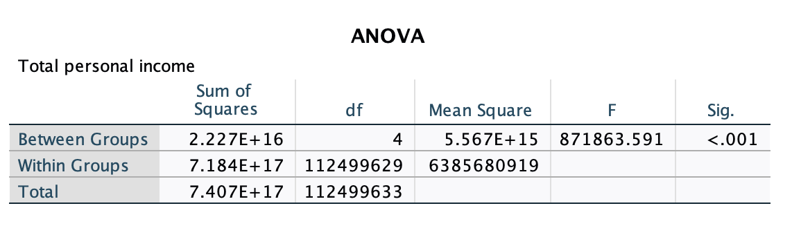
This is the ANOVA part. The E+15, E+16, and E+17 are for scientific notation (e.g., 2.227E+16 is for 2.227x10¹⁶). Because these are sums of squares, they tend to be big numbers. Our F-statistic is 871,863.59. Based on the F-statistic, the number of groups, and the sample size, our p-value is <0.001.
1 - 0.001 = 0.999 = 99.9% OR 100% - 0.1% = 99.9%
That means we can be over 99.9% confident that we can reject our null and accept our alternative hypothesis. We are over 99% confident that not all racial groups have the same mean income.
But that doesn't tell us much!
There are "post hoc" tests that can be used to test for which groups have significantly different means from which groups, but there are a lot of options. Tukey is the most common. You could click on the post hoc button in the One-Way ANOVA box:
and then select the method you are going to use:
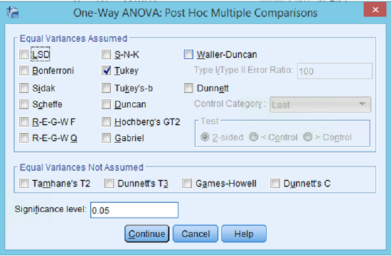
or you could add this to the last line of your ANOVA syntax:
/POSTHOC=TUKEY ALPHA(0.05).
However, when we ran the ANOVA, we also ran descriptive statistics, including confidence intervals. Rather than use a post-hoc test, we're just going to turn back to our skills from Chapter 6 and compare the racial groups based on their confidence intervals.
I generated a means plot with the ANOVA output. Here's what it looks like:
This tracks sample means. I find the lines distracting and inappropriately showing movement between categories, so I usually delete the lines and make the points bigger.
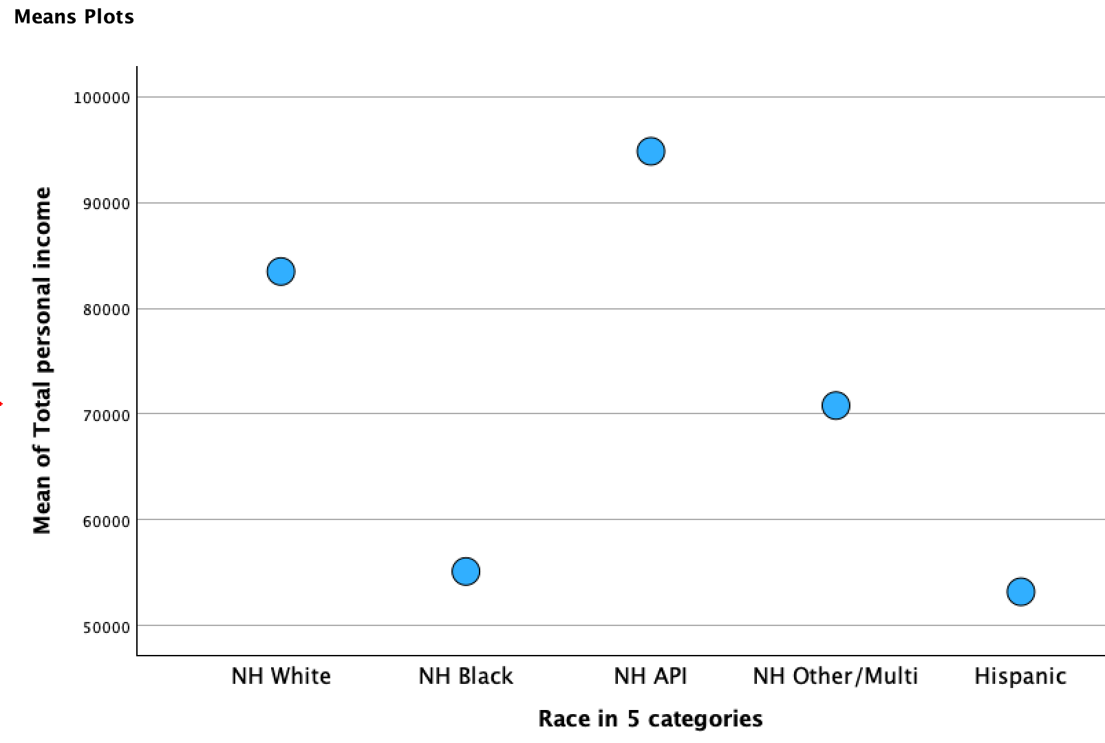
This is a quick visual way to get a sense of where the sample means are for each category in relation to one another.
Here is the rest of the descriptives output:
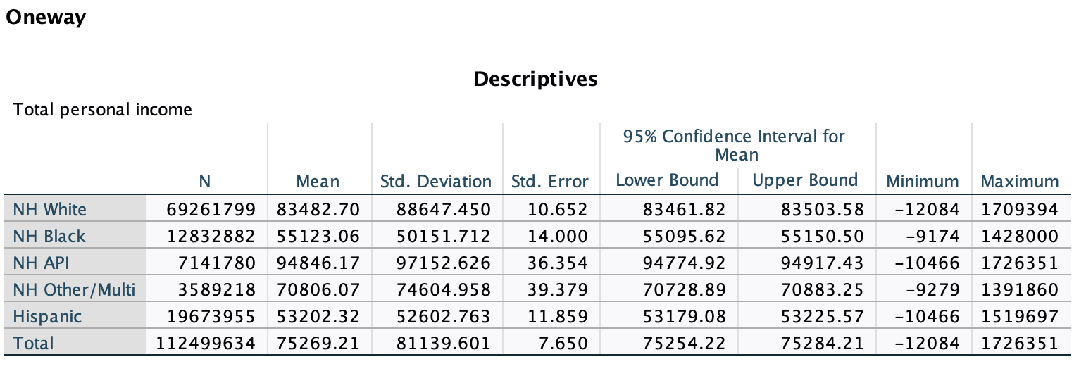
Because this is such a large dataset, we have very narrow confidence intervals, and so none of the confidence intervals overlap. Each racial group has a significantly different mean than each other racial group. We are over 95% confident that all the population means are different.
While all the means were different here, it doesn't have to be for the p-value in our ANOVA statistical test to be <0.05. If p<0.05, it just means that at least ONE group mean is different from at least ONE other group mean. The rest could all be the same.
Now that we've determined that they are significantly different, let's look at whether or not they are substantively different.
At the 95% confidence level:
- Hispanic upper bound $53,226; NH Black lower bound: $55,096. At least $1,870 apart.
- NH Black upper bound: $55,151; NH Other/Multi lower bound: $70,729. Over $10,000 apart. (Hispanic more)
- NH Other/Multi upper bound: $70,883; NH White lower bound: $83,462. Over $10,000 apart. (Hispanic and NH Black more)
- NH White upper bound: $83,504; NH API lower bound: $94,775. Over $10,000 apart. (Hispanic, NH Black, and NH Other/Multi more)
You could argue either way about the difference between the mean income for Hispanic and NH Black workers, but all the other group pairings are substantively different from one another.
Is it causal?
This is asking whether race has an impact or effect on variation in income. I would argue it is causal. We have a significant and substantive relationship. The causal order makes sense: while race might cause differences in pay, it would not make sense for how much one earns to change someone's race. Race is a relatively stable social location and racism could impact the kinds of jobs and pay workers of different racial groups earn. Theoretically, it makes sense that race impacts mean earnings. There is a robust body of sociological scholarship explaining various reasons for the racial pay gap (e.g., outright discrimination, wealth and opportunity gaps, segregation, etc.). There are no other preceding variables that would explain away this relationship.