Given that so few organisms ever become fossilized, any anthropologist or fossil hunter will tell you that finding a fossil is extremely exciting. But this is just the beginning of a fantastic mystery. With the creative application of scientific methods and deductive reasoning, a great deal can be learned about the fossilized organism and the environment in which it lived, leading to enhanced understanding of the world around us.
Dating Methods
Context is a crucial concept in paleoanthropology and archaeology. Objects and fossils are interesting in and of themselves, but without context there is only so much we can learn from them. One of the most important contextual pieces is the dating of an object or fossil. By being able to place it in time, we can compare it more accurately with other contemporary fossils and artifacts or we can better analyze the evolution of a fossil species or artifacts. To answer the question “How do we know what we know?,” you have to know how archaeologists and paleoanthropologists establish dates for artifacts, fossils, and sites.
Though accurate dating is important for context and analysis, we must consider the impact. Many of the chronometric dating methods used by anthropologists require the removal of small samples from artifacts, bones, soils, and rock. Thus these techniques are considered destructive. How much of an artifact are you willing to destroy to get your date? Sharon Clough, a Senior Environmental Officer at Cotswold Archaeology, addressed this issue in a case study from her research. She stated that “the benefit of a date did not outweigh the destruction of a valuable and finite resource” (Clough 2020). The resource in question was human remains. When considering our dating options, we want to be sure that we do as little harm as possible, especially in the case of human remains (read more about this issue in the Special Topic box, “Necropolitics”).
Dating techniques are divided into two broad categories: relative dating methods and chronometric (sometimes called absolute) dating methods.
Relative Dating
Relative dating methods are used first because they rely on simple observational skills. In the 1820s, Christian Jürgensen Thomsen at the National Museum of Denmark in Copenhagen developed the “three-age” system still used in European archaeology today (Feder 2017, 17). He categorized the artifacts at the museum based on the idea that simpler tools and materials were most likely older than more complex tools and materials. Stone tools must predate metal tools because they do not require special technology to develop. Copper and bronze tools must predate iron because they can be smelted or worked at lower temperatures, etc. Based on these observations, he categorized the artifacts into Stone Age, Bronze Age, and Iron Age.
The restriction of relative dating is that you don’t know specific dates or how much time passed between different sites or artifacts. You simply know that one artifact or fossil is older than another. Thomsen knew that Stone Age artifacts were older than Bronze Age artifacts, but he couldn’t tell if they were hundreds of years older or thousands of years older. The same is true with fossils that have differences of ages into the hundreds of millions of years.
The first relative dating technique is stratigraphy (Figure 7.20). You might have already heard this term if you have watched documentaries on archaeological excavations. That’s because this method is still being used today. It provides a solid foundation for other dating techniques and gives important context to artifacts and fossils found at a site.
Stratigraphy is based on the Law of Superposition first proposed by Nicholas Steno in 1669 and further explored by James Hutton (the previously mentioned “Father” of Deep Time). Essentially, superposition tells us that things on the bottom are older than things on the top (Williams 2004, 28). Notice on Figure 7.20 that there are distinctive layers piled on top of each other. It stands to reason that each layer is older than the one immediately on top of it (Hester et al. 1997, 338). Think of a pile of laundry on the floor. Over the course of a week, as dirty clothes get tossed on that pile, the shirt tossed down on Monday will be at the bottom of the pile while the shirt tossed down on Friday will be at the top. Assuming that the laundry pile was undisturbed throughout the week, if the clothes were picked up layer by layer, the clothing choices that week could be reconstructed in the order that they were worn.
Another relative dating technique is biostratigraphy. This form of dating looks at the context of a fossil or artifact and compares it to the other fossils and biological remains (plant and animal) found in the same stratigraphic layers. For instance, if an artifact is found in the same layer as wooly mammoth remains, you know that it must date to around the last ice age, when wooly mammoths were still abundant on Earth. In the absence of more specific dating techniques, early archaeologists could prove the great antiquity of stone tools because of their association with extinct animals. The application of this relative dating technique in archaeology was used at the Folsom site in New Mexico. In 1927, a stone spear point was discovered embedded in the rib of an extinct species of bison. Because of the undeniable association between the artifact and the ancient animal, there was scientific evidence that people had occupied the North American continent since antiquity (Cook 1928).
Similar to biostratigraphic dating is cultural dating (Figure 7.21). This relative dating technique is used to identify the chronological relationships between human-made artifacts. Cultural dating is based on artifact types and styles (Hester et al. 1997, 338). For instance, a pocket knife by itself is difficult to date. However, if the same pocket knife is discovered surrounded by cassette tapes and VHS tapes, it is logical to assume that the artifact came from the late 20th century like the cassette and VHS tapes. The pocket knife could not be dated earlier than the late 20th century because the tapes were made no earlier than 1977. In the Thomsen example above, he was able to identify a relative chronology of ancient European tools based on the artifact styles, manufacturing techniques, and raw materials. Cultural dating can be used with any human-made artifacts. Both cultural dating and biostratigraphy are most effective when researchers are already familiar with the time periods for the artifacts and animals. They are still used today to identify general time periods for sites.
Chemical dating was developed in the 19th century and represents one of the early attempts to use soil composition and chemistry to date artifacts. A specific type of chemical dating is fluorine dating, and it is commonly used to compare the age of the soil around bone, antler, and teeth located in close proximity (Cook and Ezra-Cohn 1959; Goodrum and Olson 2009). While this technique is based on chemical dating, it only provides the relative dates of items rather than their absolute ages. For this reason, fluorine dating is considered a hybrid form of relative and chronometric dating methods (which will be discussed next).
Soils contain different amounts of chemicals, and those chemicals, such as fluorine, can be absorbed by human and animal bones buried in the soil. The longer the remains are in the soil, the more fluorine they will absorb (Cook and Ezra-Cohn 1959; Goodrum and Olson 2009). A sample of the bone or antler can be processed and measured for its fluorine content. Unfortunately, this absorption rate is highly sensitive to temperature, soil pH, and varying fluorine levels in local soil and groundwater (Goodrum and Olson 2009; Haddy and Hanson 1982). This makes it difficult to get an accurate date for the remains or to compare remains between two sites. However, this technique is particularly useful for determining whether different artifacts come from the same burial context. If they were buried in the same soil for the same length of time, their fluorine signatures would match.
Chronometric Dating
Unlike relative dating methods, chronometric dating methods provide specific dates and time ranges. Many of the chronometric techniques we will discuss are based on work in other disciplines such as chemistry and physics. The modern developments in studying radioactive materials are accurate and precise in establishing dates for ancient sites and remains.
Many of the chronometric dating methods are based on the measurement of radioactive decay of particular elements. Elements are materials that cannot be broken down into more simple materials without losing their chemical identity (Brown et al. 2018, 48). Each element consists of an atom that has a specific number of protons (positively charged particles) and electrons (negatively charged particles) as well as varying numbers of neutrons (particles with no charge). The protons and neutrons are located in the densely compacted nucleus of the atom, but the majority of the volume of an atom is space outside the nucleus around which the electrons orbit (see Figure 7.22).
Elements are classified based on the number of protons in the nucleus. For example, carbon has six protons, giving it an atomic number 6. Uranium has 92 protons, which means that it has an atomic number 92. While the number of protons in the atom of an element do not vary, the number of neutrons may. Atoms of a given element that have different numbers of neutrons are known as isotopes.
The majority of an atom’s mass is determined by the protons and neutrons, which have more than a thousand times the mass of an electron. Due to the different numbers of neutrons in the nucleus, isotopes vary by nuclear/atomic weight (Brown et al. 2018, 94). For instance, isotopes of carbon include carbon 12 (12C), carbon 13 (13C), and carbon 14 (14C). Carbon always has six protons, but 12C has six neutrons whereas 14C has eight neutrons. Because 14C has more neutrons, it has a greater mass than 12C (Brown et al. 2018, 95).
Most isotopes in nature are considered stable isotopes and will remain in their normal structure indefinitely. However, some isotopes are considered unstable isotopes (sometimes called radioisotopes) because they spontaneously release energy and particles, transforming into stable isotopes (Brown et al. 2018, 946; Flowers et al. 2018, section 21.1). The process of transforming the atom by spontaneously releasing energy is called radioactive decay. This change occurs at a predictable rate for nearly all radioisotopes of elements, allowing scientists to use unstable isotopes to measure time passage from a few hundred to a few billion years with a large degree of accuracy and precision.
The leading chronometric method for archaeology is radiocarbon dating (Figure 7.23). This method is based on the decay of 14C, which is an unstable isotope of carbon. It is created when nitrogen 14 (14N) interacts with cosmic rays, which causes it to capture a neutron and convert to 14C. Carbon 14 in our atmosphere is absorbed by plants during photosynthesis, a process by which light energy is turned into chemical energy to sustain life in plants, algae, and some bacteria. Plants absorb carbon dioxide from the atmosphere and use the energy from light to convert it into sugar that fuels the plant (Campbell and Reece 2005, 181–200). Though 14C is an unstable isotope, plants can use it in the same way that they use the stable isotopes of carbon.
Animals get 14C by eating the plants. Humans take it in by eating plants and animals. After death, organisms stop taking in new carbon, and the unstable 14C will begin to decay. Carbon 14 has a half-life of 5,730 years (Hester et al. 1997, 324). That means that in 5,730 years, half the amount of 14C will convert back into 14N. Because the pattern of radioactive decay is so reliable, we can use 14C to accurately date sites up to 55,000 years old (Hajdas et al. 2021). However, 14C can only be used on the remains of biological organisms. This includes charcoal, shell, wood, plant material, and bone. This method involves destroying a small sample of the material. Earlier methods of radiocarbon dating required at least 1 gram of material, but with the introduction of accelerator mass spectrometry (AMS), sample sizes as small as 1 milligram can now be used (Hajdas et al. 2021). This significantly reduces the destructive nature of this method.
The use of radiocarbon dating at Denisova Cave in modern-day Russia revealed an astounding find, the first dated first-generation individual with a Neanderthal mother and Denisovan father. Vivian Slon and colleagues (2018) sequenced the genome, which revealed the individual’s hybrid genetic background, and radiocarbon dated the remains, revealing the sub-adult was over 50,000 years old (Slon et al. 2018).
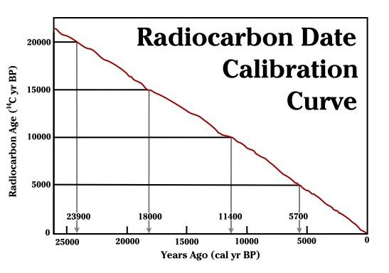
As mentioned before, 14C is unstable and ultimately decays back into 14N. This decay is happening at a constant rate (even now, inside your own body!). However, as long as an organism is alive and taking in food, 14C is being replenished in the body. As soon as an organism dies, it no longer takes in new 14C. We can then use the rate of decay to measure how long it has been since the organism died (Hester et al. 1997, 324). However, the amount of 14C in the atmosphere is not stable over time. It fluctuates based on changes to the earth’s magnetic field and solar activity. In order to turn 14C results into accurate calendar years, they must be calibrated using data from other sources. Annual tree rings (see discussion of dendrochronology below), foraminifera from stratified marine sediments, and microfossils from lake sediments can be used to chart the changes in 14C as “calibration curves.” The radiocarbon date obtained from the sample is compared to the established curve and then adjusted to reflect a more accurate calendar date (see Figure 7.24). The curves are updated over time with more data so that we can continue to refine radiocarbon dates (Törnqvist et al. 2016). The most recent calibration curves were released in 2020 and may change the dates for some existing sites by hundreds of years (Jones 2020).
Figure 7.24: This is a simplified example of a calibration curve, showing how the radiocarbon age (y axis) is compared with the calibration curve to produce calibrated dates (x axis). Credit: Radiocarbon Date Calibration Curve by HowardMorland is under a CC BY-SA 3.0 License. [Based on information from Reimer et al. 2004. Radiocarbon 46: 1029-58.] [Image Description].
As you will see in the hominin chapters (Chapters 9–12), 55,000 years is only a tiny fragment of human evolutionary history. It is insignificant in the context of the age of our planet. In order to date even older fossils, other methods are necessary.
Potassium-argon (K-Ar) dating and argon-argon (Ar-Ar) dating can reach further back into the past than radiocarbon dating. Used to date volcanic rock, these techniques are based on the decay of unstable potassium 40 (40K) into argon 40 (40Ar) gas, which gets trapped in the crystalline structures of volcanic material. It is a method of indirect dating. Instead of dating the fossil itself, K-Ar and Ar-Ar dates volcanic layers around the fossil. It will tell you when the volcanic eruption that deposited the layers occurred. This is where stratigraphy becomes important. The date of the surrounding layers can give you a minimum and maximum age of the fossil based on where it is in relation to those layers. This technique was used at Gesher Benot Ya’aqo in the Jordan Valley, dating early stratigraphic deposits of basalt flows to 100,000 years old (Bar-Yosef and Belmaker 2011). The site is unique because early layers of occupation with an Acheulean handaxe industry were made primarily of basalt, which is an uncommon material for this tool technology (see Chapter 10 for a full discussion of this tool technology). The benefit of this dating technique is that 40K has a half-life of circa 1.3 billion years, so it can be used on sites as young as 100 kya and as old as the age of Earth. As you will see in later chapters, it is particularly useful in dating early hominin sites in Africa (Michels 1972, 120; Renfrew and Bahn 2016, 155). Another benefit to this technique is that it does not damage precious fossils because the samples are taken from the surrounding rock instead. However, this method is not without its flaws. A study by J. G. Funkhouser and colleagues (1966) and Raymond Bradley (2015) demonstrated that igneous rocks with fluid inclusions, such as those found in Hawai‘i, can release gasses including radiogenic argon when crushed, leading to incorrectly older dates. This is an example of why it is important to use multiple dating methods in research to detect anomalies.
Uranium series dating is based on the decay chain of unstable isotopes of uranium. It uses mass spectrometry to detect the ratios of uranium 238 (238U), uranium 234(234U), and thorium 230 (230Th) in carbonates (Wendt et al. 2021). Thorium accumulates in the carbonate sample through radiometric decay. Thus, the age of the sample is calculated from the difference between a known initial ratio and the ratio present in the sample to be dated. This makes uranium series ideal for dating carbonate rich deposits such as carbonate cements from glacial moraine deposits, speleothems (deposits of secondary minerals that form on the walls, floors, and ceilings of caves, like stalactites and stalagmites), marine and lacustrine carbonates from corals, caliche, and tufa, as well as bones and teeth (University of Arizona, n.d.; van Calsteren and Thomas 2006). Due to the timing of the decay process, this dating technique can be used from a few years up to 650k (Wendt et al. 2021). Since many early hominin sites occur in cave environments, this dating technique can be very powerful. This method has also been used to develop more accurate calibration curves for radiocarbon dating. However, the accuracy of this method depends on knowing the initial ratios of the elements and ruling out possible contamination (Wendt et al. 2021). It also involves the destruction of a small sample of material.
Fission track dating is another useful dating technique for sites that are millions of years old. This is based on the decay of radioactive uranium 238 (238U). The unstable atom of 238U fissions at a predictable rate. The fission takes a lot of energy and causes damage to the surrounding rock. For instance, in volcanic glasses we can see this damage as trails in the glass. Researchers in the lab take a sample of the glass and count the number of fission trails using an optical microscope. As 238U has a half-life of 4,500 million years, it can be used to date rock and mineral material starting at just a few decades and extending back to the age of Earth. As with K-Ar, archaeologists are not dating artifacts directly. They are dating the layers around the artifacts in which they are interested (Laurenzi et al. 2007).
Luminescence dating, which includes thermoluminescence and a related technique called optically stimulated luminescence, is based on the naturally occurring background radiation in soils. Pottery, baked clay, and sediments that include quartz and feldspar are bombarded by radiation from the soils surrounding it. Electrons in the material get displaced from their orbit and trapped in the crystalline structure of the pottery, rock, or sediment. When a sample of the material is heated to 500°C (thermoluminescence) or exposed to particular light wavelengths (optically stimulated luminescence) in the laboratory, this energy gets released in the form of light and heat and can be measured (Cochrane et al. 2013; Renfrew and Bahn 2016, 160). You can use this method to date artifacts like pottery and burnt flint directly. When attempting to date fossils, you may use this method on the crystalline grains of quartz and feldspar in the surrounding soils (Cochrane et al. 2013). The important thing to remember with this form of dating is that heating the artifact or soils will reset the clock. The method is not necessarily dating when the object was last made or used but when it was last heated to 500°C or more (pottery) or exposed to sunlight (sediments). Luminescence dating can be used on sites from less than 100 years to over 100,000 years (Duller 2008, 4). As with all archaeological data, context is crucial to understanding the information.
Like thermoluminescence dating, electron spin resonance dating is based on the measurement of accumulated background radiation from the burial environment. It is used on artifacts and rocks with crystalline structures, including tooth enamel, shell, and rock—those for which thermoluminescence would not work. The radiation causes electrons to become dislodged from their normal orbit. They become trapped in the crystalline matrix and affect the electromagnetic energy of the object. This energy can be measured and used to estimate the length of time in the burial environment. This technique works well for remains as old as two million years (Carvajal et al. 2011, 115–116). It has the added benefit of being nondestructive, which is an important consideration when dealing with irreplaceable material.
Not all chronometric dating methods are based on unstable isotopes and their rates of decay. There are several other methods that make use of other natural biological and geologic processes. One such method is known as dendrochronology (Figure 7.25), which is based on the natural growth patterns of trees. Trees create concentric rings as they grow; the width of those rings depends on environmental conditions and season. The age of a tree can be determined by counting its rings, which also show records of rainfall, droughts, and forest fires.
Tree rings can be used to date wood artifacts and ecofacts from archaeological sites. This first requires the creation of a profile of trees in a particular area. The Laboratory of Tree-Ring Research at the University of Arizona has a comprehensive and ongoing catalog of tree profiles (see University of Arizona n.d.). Archaeologists can then compare wood artifacts and ecofacts with existing timelines, provided the tree rings are visible, and find where their artifacts fit in the pattern. Dendrochronology has been in use since the early 20th century (Dean 2009, 25). The Northern Hemisphere chronology stretches back nearly 14,000 years (Reimer et al. 2013, 1870) and has been used successfully to date southwestern U.S. sites such as Pueblo Bonito and Aztec Ruin (Dean 2009, 26). Dendrochronological evidence has helped calibrate radiocarbon dates and even provided direct evidence of global warming (Dean 2009, 26–27).
In Australia, dendrochronology, along with other environmental reconstruction methods, has been used to show that the Indigenous people had sophisticated land management systems before the arrival of British invaders. According to the work of Michael-Shawn Fletcher and colleagues (2021), there was a significant encroachment of the rainforests and tree species into grasslands after the British invasion. Prior to this time, Indigenous people managed the landscape through controlled burns at regular intervals. This practice created climate-resistant grasslands that were biodiverse and provided predictable food supplies for humans and other animals. Under European land management, there have been negative impacts on biodiversity and climate resilience and an increase in catastrophic wildfires (Fletcher et al. 2021).
This dating method does have its difficulties. Some issues are interrupted ring growth, microclimates, and species growth variations. This is addressed through using multiple samples, statistical analysis, and calibration with other dating methods. Despite these limitations, dendrochronology can be a powerful tool in dating archaeological sites (Hillam et al. 1990; Kuniholm and Striker 1987).
Environmental Reconstruction
As you read in Chapter 2, Charles Darwin, Jean-Baptiste Lamarck, Alfred Russel Wallace, and others recognized the importance of the environment in shaping the evolutionary course of animal species. To understand what selective processes might be shaping evolutionary change, we must be able to reconstruct the environment in which the organism was living.
One of the ways to do that is to look at the plant species that lived in the same time range as the species in which you are interested. One way to identify ancient flora is to analyze sediment cores from water and other protected sources. Pollen gets released into the air and some of that pollen will fall on wetlands, lakes, caves, and so forth. Eventually it sinks to the bottom of the lake and forms part of the sediment. This happens year after year, so subsequent layers of pollen build up in an area, creating strata. By taking a core sample and analyzing the pollen and other organic material, an archaeologist can build a timeline of plant types and see changes in the vegetation of the area (Hester et al. 1997, 284). This can even be done over large areas by studying ocean bed cores, which accumulate pollen and dust from large swaths of neighboring continents.
While sediment coring is one of the more common ways to reconstruct past environments, there are a few other methods. These have been recently employed at Holocene Lake Ivanpah, a paleolake that straddles the California and Nevada border in the United States. This lake was originally thought to have been completely dry around 9,300–7,800 kya (Sims and Spaulding 2017). However, analyzing core samples using soil identification, sediment chemistry, subsurface stratigraphy, and geomorphology (the study of the physical characteristics of the Earth’s surface) revealed deposition of three recent lake fillings during this period in the forms of additional hardpan, or lake bottom, playas, bedded or layered fine-grained (wetland) sediments, and buried beaches below the surface (Sims and Spaulding 2017; Spaulding and Sims 2018). These discoveries are important because they have not been integrated into interpretation of the local archaeological record, as it was assumed that the lake had been dry for thousands of years. Sedimentological analyses such as coring and those listed above can provide great insight into past climates and are accomplished in a minimally destructive way.
Another way of reconstructing past environments is by using stable isotopes. Unlike unstable isotopes, stable isotopes remain constant in the environment throughout time. Plants take in the isotopes through photosynthesis and ground water absorption. Animals take in isotopes by drinking local water and eating plants. Stable isotopes can be powerful tools for identifying where an organism grew up and what kind of food the organism ate throughout its life. They can even be used to identify global temperature fluctuations.
Global Temperature Reconstruction
Oxygen isotopes are a powerful tool in tracking global temperature fluctuations throughout time. The isotopes of Oxygen 18 (18O) and Oxygen 16 (16O) occur naturally in Earth’s water. Both are stable isotopes, but 18O has a heavier atomic weight. In the normal water cycle, evaporation takes water molecules from the surface to the atmosphere. Because 16O is lighter, it is more likely to be part of this evaporation process. The moisture gathers in the atmosphere as clouds that eventually may produce rain or snow and release the water back to the surface of the planet. During cool periods like glacial periods (ice ages), the evaporated water often comes down to Earth’s surface as snow. The snow piles up in the winter but, because of the cooler summers, does not melt off. Instead, it gets compacted and layered year after year, eventually resulting in large glaciers or ice sheets covering parts of Earth. Since 16O, with the lighter atomic weight, is more likely to be absorbed in the evaporation process, it gets locked up in glacier formation. The waters left in oceans would have a higher ratio of 18O during these periods of cooler global temperatures (Potts 2012, 154–156; see Figure 7.26).
The microorganisms that live in the oceans, foraminifera, absorb the water from their environment and use the oxygen isotopes in their body structures. When these organisms die, they sink to the ocean floor, contributing to the layers of sediment. Scientists can extract these ocean cores and sample the remains of foraminifera for their 18O and 16O ratios. These ratios give us a good approximation of global temperatures deep into the past. Cooler temperatures indicate higher ratios of 18O (Potts 2012, 154–156).
Diet Reconstruction
You may be familiar with the saying “you are what you eat.” When it comes to your teeth and bones, this adage is literal. Stable isotopes can also be used to reconstruct animal diet and migration patterns. Living organisms absorb elements from ingested plants and water. These elements are used in tissues like bones, teeth, skin, hair, and so on. By analyzing the stable isotopes in the bones and teeth of humans and other animals, we can identify the types of food they ate at different stages of their lives.
Plants take in carbon dioxide from the atmosphere during photosynthesis. We’ve already discussed this using the example of the unstable isotope 14C; however, this absorption also takes place with the stable isotopes of 12C and 13C. During photosynthesis, some plants incorporate carbon dioxide as a three-carbon molecule (C3 plants) and some as a four-carbon molecule (C4 plants). On the one hand, C3 plants include certain types of trees and shrubs that are found in relatively wet environments and have lower ratios of 13C compared to 12C. C4 plants, on the other hand, include plants from drier environments like savannahs and grasslands. C4 plants have higher ratios of 13C to 12C than C3 plants (Renfrew and Bahn 2016, 312). These ratios remain stable as you go up the food chain. Therefore, you can analyze the bones and teeth of an animal to identify the 13C/12C ratios and identify the types of plants that animal was eating.
The ratios of stable nitrogen isotopes 15N and 14N can also give information about the diet of fossilized or deceased organisms. Though initially absorbed from water and soils by plants, the nitrogen ratios change depending on the primary diet of the organism. An animal who has a mostly vegetarian diet will have lower ratios of 15N to 14N, while those further up the food chain, like carnivores, will have higher ratios of 15N. Interestingly, breastfeeding infants have a higher nitrogen ratio than their mothers, because they are getting all of their nutrients through their mother’s milk. So nitrogen can be used to track life events like weaning (Jay et al. 2008, 2). A marine versus terrestrial diet will also affect the nitrogen signatures. Terrestrial diets have lower ratios of 15N than marine diets. In the course of human evolution, this type of analysis can help us identify important changes in human nutrition. It can help anthropologists figure out when meat became a primary part of the ancient human diet or when marine resources began to be used. The ratios of stable nitrogen isotopes can also be used to determine a change in status, as in the case of the Llullaillaco children (the “ice mummies”) found in the Andes Mountains. For instance, the nitrogen values in hair from the Llullaillaco Maiden showed a significant positive shift that is associated with increased meat consumption in the last 12 months of her life (Wilson et al. 2007). Although the two younger children had little changes in their diets in the last year of their short lives, the changes in their nitrogen values were significant enough to suggest that the improvement in their diets may have been attributed to the Incas’ desire to sacrifice healthy, high-status children” (Faux 2012, 6).
Migration
Stable isotopes can also tell us a great deal about where an individual lived and whether they migrated during their lifetime. The geology of Earth varies because rocks and soils have different amounts or ratios of certain elements in them. These variations in the ratios of isotopes of certain elements are called isotopic signatures. They are like a chemical fingerprint for a geographical region. These isotopes get into the groundwater and are absorbed by plants and animals living in that area. Elements like strontium, oxygen, and nitrogen, among others, are then used by the body to build bones and teeth. If you ate and drank local water all of your life, your bones and teeth would have the same isotopic signature as the geographical region in which you lived.
However, many people (and animals) move around during their lifetimes. Isotopic signatures can be used to identify migration patterns in organisms (Montgomery et al. 2005). Teeth develop in early childhood. If the isotopes of teeth are analyzed, these isotopes would resemble those found in the geographic area where an individual lived as a child. Bones, however, are a different story. Bones are constantly changing throughout life. Old cells are removed and new cells are deposited to respond to growth, healing, activity change, and general deterioration. Therefore, the isotopic signature of bones will reflect the geographical area in which an individual spent the last seven to ten years of life. If an individual has different isotopic signatures for their bones and teeth, it could indicate a migration some time during their life after childhood.
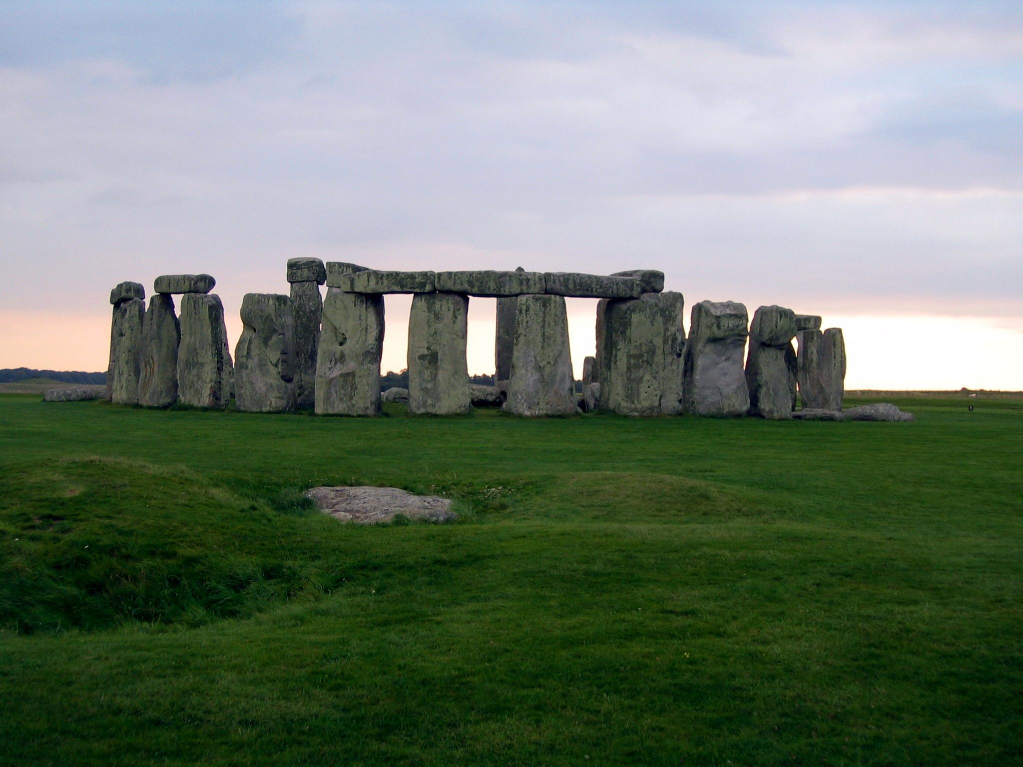
Figure 7.27: Stonehenge continues to provide clues to its mysterious existence with recent research using isotope ratios. Credit: Stonehenge (Figure 7.37) by Sarah S. King is under a CC BY-NC 4.0 License.
Recent work involving stable isotope analysis has been done on the cremation burials from Stonehenge, in Wessex, England (Figure 7.27). Much of the archaeological work at Stonehenge in the past focused on the building and development of the monument itself. That is partly because most of the burials at the monument were cremated remains, which are difficult to study because of their fragmentary nature and the chemical alterations that bone and teeth undergo when heated. The cremation process complicates the oxygen and carbon isotopes. However, the researchers determined that strontium would not be affected by heating and could still be analyzed in cranial fragments. Using the remains of 25 individuals, they compared their strontium signatures to the geology of Wessex and other regions of the UK. Fifteen of those individuals had strontium signatures that matched the local geology. This means that in the last ten or so years of their lives, they lived and ate food from around Stonehenge. However, ten of the individuals did not match the local geologic signature. These individuals had strontium ratios more closely aligned with the geology of west Wales. Archaeologists find this particularly interesting because in the early phases of Stonehenge’s construction, the smaller “blue stones” were brought 200 km from Wales in a feat of early engineering. These larger regional connections show that Stonehenge was not just a site of local importance. It dominated a much larger region of influence and drew people from all over ancient Britain (Snoeck et al. 2018).
In 2007, cave divers exploring the Sistema Sac Actun in the Yucatán Peninsula in Mexico (see Figure 7.28 and 7.29) discovered the bones of a 15- to 16-year-old female human along with the bones of various extinct animals from the Pleistocene (Collins et al. 2015). The site was named Hoyo Negro (“Black Hole”). The human bones belonged to a Paleo-American, later named “Naia” after a Greek water nymph. Examination of the partially fossilized remains revealed a great deal about Naia’s life, and the radiocarbon dating of her tooth enamel indicated that she lived some 13,000 years ago (Chatters et al. 2014). Naia’s arms were not overly developed, so her daily activities did not involve heavy carrying or grinding of grain or seeds. Her legs, however, were quite muscular, implying that Naia was used to walking long distances. Naia’s teeth and bones indicate habitually poor nutrition. There is evidence of violent injury during the course of Naia’s life from a healed spiral fracture of her left forearm. Naia also suffered from tooth decay and osteoporosis even though she appeared young and undersized. Dr. Jim Chatters hypothesizes that Naia entered the cave at a time when it was not flooded, probably looking for water. She may have become disoriented and fell off a high ledge to her death. The trauma to her pelvis is consistent with such an injury (Watson 2017).
Naia’s skeleton is remarkably complete given its age. As divers were able to locate her skull, Naia’s physical appearance in life could be interpreted. Surprisingly, in examining the skull, it was determined that Naia did not resemble modern Indigenous peoples in the region. However, the mitochondrial DNA (mtDNA) recovered from a tooth indicates that Naia shares her DNA with modern Indigenous peoples (Chatters et al. 2014). Though Naia’s burial environment made chemical analysis difficult, researchers were able to recover carbon isotopes from her remains. The isotopes from Naia’s tooth enamel suggest a diet of “cool-season grasses and/or broad-leaf vegetation” (Chatters et al. 2022, 68). Naia’s teeth also displayed numerous dental caries and only light dental wear. Coupled with the isotopic data, she likely had a “softer, more sugar-rich diet” (Chatters et al. 2022, 68).
Figure 7.29: A diagram of the Sistema Sac Actun and the Hoyo Negro cenote where Naia rested underwater for roughly 13,000 years. The illustration depicts a cenote or hole in the ground leading to a long, narrow tunnel, ending in a large cavern. The cavern and tunnel are both filled with water. Credit: Hoyo Negro cenote (Figure 7.39) original to Explorations: An Open Invitation to Biological Anthropology by Mary Nelson is under a CC BY-NC 4.0 License.
Summary
With a timeline that extends back some 4.6 billion years, Earth has witnessed continental drift, environmental changes, and a growing complexity of life. Fossils, the mineralized remains of living organisms, provide physical evidence of life and the environment on the planet over the course of billions of years. In order to better understand the fossil record, anthropologists rely on the collaboration of numerous academic fields and disciplines. Anthropologists use a variety of scientific methods, both relative and chronometric, to analyze fossils to determine age, origins, and migration patterns as well as to provide insight into the health and diet of the fossilized organism. While each method has its advantages, disadvantages, and limited applications, these tools enable anthropologists to theorize how all living organisms evolved, including the evolution of early humans into modern humans, H. sapiens. The fossil record is far from complete, but our expanding understanding of the fossil context, with exciting new discoveries and improved scientific methods, enables us to document the history of our planet and the evolution of life on Earth.