The cost structure for the production of snowboards at Black Diamond is illustrated in Table 8.2. Employees are skilled and are paid a weekly wage of $1,000. The cost of capital is $3,000 and it is fixed, which means that it does not vary with output. As in Table 8.1, the number of employees and the output are given in the first two columns. The following three columns define the capital costs, the labour costs, and the sum of these in producing different levels of output. We use the terms fixed, variable, and total costs to define the cost structure of a firm. Fixed costs do not vary with output, whereas variable costs do, and total costs are the sum of fixed and variable costs. To keep this example as simple as possible, we will ignore the cost of raw materials. We could add an additional column of costs, but doing so will not change the conclusions.
Table 8.2 Snowboard production costs
| Workers |
Output |
Capital |
Labour |
Total |
Average |
Average |
Average |
Marginal |
| |
|
cost |
cost |
costs |
fixed |
variable |
total |
cost |
| |
|
fixed |
variable |
|
cost |
cost |
cost |
|
| 0 |
0 |
3,000 |
0 |
3,000 |
|
|
|
|
| 1 |
15 |
3,000 |
1,000 |
4,000 |
200.0 |
66.7 |
266.7 |
66.7 |
| 2 |
40 |
3,000 |
2,000 |
5,000 |
75.0 |
50.0 |
125.0 |
40.0 |
| 3 |
70 |
3,000 |
3,000 |
6,000 |
42.9 |
42.9 |
85.7 |
33.3 |
| 4 |
110 |
3,000 |
4,000 |
7,000 |
27.3 |
36.4 |
63.6 |
25.0 |
| 5 |
145 |
3,000 |
5,000 |
8,000 |
20.7 |
34.5 |
55.2 |
28.6 |
| 6 |
175 |
3,000 |
6,000 |
9,000 |
17.1 |
34.3 |
51.4 |
33.3 |
| 7 |
200 |
3,000 |
7,000 |
10,000 |
15.0 |
35.0 |
50.0 |
40.0 |
| 8 |
220 |
3,000 |
8,000 |
11,000 |
13.6 |
36.4 |
50.0 |
50.0 |
| 9 |
235 |
3,000 |
9,000 |
12,000 |
12.8 |
38.3 |
51.1 |
66.7 |
| 10 |
240 |
3,000 |
10,000 |
13,000 |
12.5 |
41.7 |
54.2 |
200.0 |
Fixed costs are costs that are independent of the level of output.
Variable costs are related to the output produced.
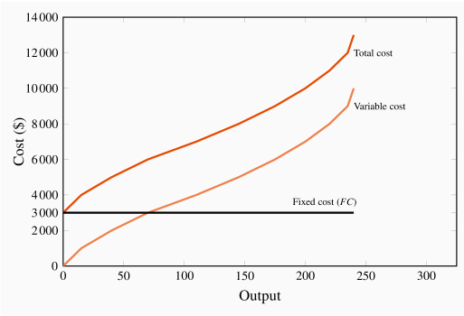
Total cost is the sum of fixed cost and variable cost.
Total costs are illustrated in Figure 8.3 as the vertical sum of variable and fixed costs. For example, Table 8.2 indicates that the total cost of producing 220 units of output is the sum of $3,000 in fixed costs plus $8,000 in variable costs. Therefore, at the output level 220 on the horizontal axis in Figure 8.3, the sum of the cost components yields a value of $11,000 that forms one point on the total cost curve. Performing a similar calculation for every possible output yields a series of points that together form the complete total cost curve.
Average costs are given in the next three columns of Table 8.2. Average cost is the cost per unit of output, and we can define an average cost corresponding to each of the fixed, variable, and total costs defined above. Average fixed cost (AFC) is the total fixed cost divided by output; average variable cost (AVC) is the total variable cost divided by output; and average total cost (ATC) is the total cost divided by output.
| AFC |
 |
| AVC |
 |
| ATC |
=AFC+AVC |
Average fixed cost is the total fixed cost per unit of output.
Average variable cost is the total variable cost per unit of output.
Average total cost is the sum of all costs per unit of output.
The productivity-cost relationship
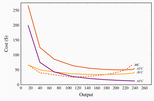
Consider the average variable cost - average product relationship, as developed in column 7 of Table 8.2; its corresponding variable cost curve is plotted in Figure 8.4. In this example, AVC first decreases and then increases. The intuition behind its shape is straightforward (and realistic) if you have understood why productivity varies in the short run: The variable cost, which represents the cost of labour, is constant per unit of labour, because the wage paid to each worker does not change. However, each worker's productivity varies. Initially, when we hire more workers, they become more productive, perhaps because they have less 'down time' in switching between tasks. This means that the labour costs per snowboard must decline. At some point, however, the law of diminishing returns sets in: As before, each additional worker is paid a constant amount, but as productivity declines the labour cost per snowboard increases.
In this numerical example the AP is at a maximum when six units of labour are employed and output is 175. This is also the point where the AVC is at a minimum. This maximum/minimum relationship is also illustrated in Figures 8.2 and 8.4.
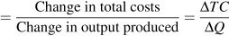
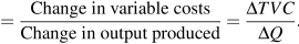
Now consider the marginal cost - marginal product relationship. The marginal cost (MC) defines the cost of producing one more unit of output. In Table 8.2, the marginal cost of output is given in the final column. It is the additional cost of production divided by the additional number of units produced. For example, in going from 15 units of output to 40, total costs increase from $4,000 to $5,000. The MC is the cost of those additional units divided by the number of additional units. In this range of output, MC is  . We could also calculate the MC as the addition to variable costs rather than the addition to total costs, because the addition to each is the same—fixed costs are fixed. Hence:
| MC |
 |
| |
 |
Marginal cost of production is the cost of producing each additional unit of output.
Just as the behaviour of the AVC curve is determined by the AP curve, so too the behaviour of the MC is determined by the MP curve. When the MP of an additional worker exceeds the MP of the previous worker, this implies that the cost of the additional output produced by the last worker hired must be declining. To summarize:
If the marginal product of labour increases, then the marginal cost of output declines;
If the marginal product of labour declines, then the marginal cost of output increases.
In our example, the  reaches a maximum when the fourth unit of labour is employed (or 110 units of output are produced), and this also is where the MC is at a minimum. This illustrates that the marginal cost reaches a minimum at the output level where the marginal product reaches a maximum.
The average total cost is the sum of the fixed cost per unit of output and the variable cost per unit of output. Typically, fixed costs are the dominant component of total costs at low output levels, but become less dominant at higher output levels. Unlike average variable costs, note that the average fixed cost must always decline with output, because a fixed cost is being spread over more units of output. Hence, when the ATC curve eventually increases, it is because the increasing variable cost component eventually dominates the declining AFC component. In our example, this occurs when output increases from 220 units (8 workers) to 235 (9 workers).
Finally, observe the interrelationship between the MC curve on the one hand and the ATC and AVC on the other. Note from Figure 8.4 that the MC cuts the AVC and the ATC at the minimum point of each of the latter. The logic behind this pattern is analogous to the logic of the relationship between marginal and average product curves: When the cost of an additional unit of output is less than the average, this reduces the average cost; whereas, if the cost of an additional unit of output is above the average, this raises the average cost. This must hold true regardless of whether we relate the MC to the ATC or the AVC.
When the marginal cost is less than the average cost, the average cost must decline;
When the marginal cost exceeds the average cost, the average cost must increase.
Notation: We use both the abbreviations  and
and  to denote average total cost. The term 'average cost' is understood in economics to include both fixed and variable costs.
Teams and services
The choice faced by the producer in the example above is slightly 'stylized', yet it still provides an appropriate rule for analyzing hiring decisions. In practice, it is quite difficult to isolate or identify the marginal product of an individual worker. One reason is that individuals work in teams within organizations. The accounting department, the marketing department, the sales department, the assembly unit, the chief executive's unit are all composed of teams. Adding one more person to human resources may have no impact on the number of units of output produced by the company in a measurable way, but it may influence worker morale and hence longer-term productivity. Nonetheless, if we consider expanding, or contracting, any one department within an organization, management can attempt to estimate the net impact of additional hires (or layoffs) on the contribution of each team to the firm's profitability. Adding a person in marketing may increase sales, laying off a person in research and development may reduce costs by more than it reduces future value to the firm. In practice this is what firms do: they attempt to assess the contribution of each team in their organization to costs and revenues, and on that basis determine the appropriate number of employees.
The manufacturing sector of the macro economy is dominated, sizewise, by the services sector. But the logic that drives hiring decisions, as developed above, applies equally to services. For example, how does a law firm determine the optimal number of paralegals to employ per lawyer? How many nurses are required to support a surgeon? How many university professors are required to teach a given number of students?
All of these employment decisions involve optimization at the margin. The goal of the decision maker is not always profit, but she should attempt to estimate the cost and value of adding personnel at the margin.