We have now described the market and firm-level equilibrium in the short run. However, this equilibrium may be only temporary; whether it can be sustained or not depends upon whether profits (or losses) are being incurred, or whether all participant firms are making what are termed normal profits. Such profits are considered an essential part of a firm's operation. They reflect the opportunity cost of the resources used in production. Firms do not operate if they cannot make a minimal, or normal, profit level. Above such profits are economic profits (also called supernormal profits), and these are what entice entry into the industry.
Recall from Chapter 7 that accounting and economic profits are different. The economist includes opportunity costs in determining profit, whereas the accountant considers actual revenues and costs. In the example developed in Section 7.2 the entrepreneur recorded accounting profit, but not economic profit. Suppose now that the numbers were slightly different, and are as defined in Table 9.2: Felicity invests $250,000 in her business in the form of capital, as before. But she now has gross revenues of $165,000 and incurs a cost of $90,000 to buy the clothing wholesale that she then sells retail. She pays herself a salary of $35,000. If these numbers represent her balance sheet, then she records an accounting profit of $40,000.
Table 9.2 Economic profits
| Sales |
|
$165,000 |
| Materials costs |
|
$90,000 |
| Wage costs |
|
$35,000 |
| Accounting profit |
|
$40,000 |
| Capital invested |
$250,000 |
|
| Implicit return on capital at 4% |
|
$10,000 |
| Additional implicit wage costs |
|
$20,000 |
| Total implicit costs |
|
$30,000 |
| Economic profit |
|
$10,000 |
Her economic profit calculation must include opportunity costs. The opportunity cost of tying up $250,000 of capital, if the interest rate is 4%, amounts to $10,000. In addition, if Felicity could earn $55,000 in her best alternative job then an additional implicit cost of $20,000 must be considered. When these two opportunity (or implicit) costs are added to the balance sheet, her profit is reduced to $10,000. This is her economic profit. If Felicity's economic profit is representative of the retail clothing sector of the economy, then that profitability should attract new entrepreneurs. Our conclusion is that this sector of the economy should experience new entrants and hence an outward shift of the supply curve. In contrast, in the numerical example considered in Section 7.2, Felicity was experiencing losses (negative economic profits), and in the longer term she would have to consider leaving the business. If she and other suppliers exited, then the market supply curve would shift back to the left – representing a reduction in supply.
The critical point in this distinction between accounting and economic cost is that the decision to enter or leave a market in the longer term is based on what the entrepreneur can earn in the wider market place. That is, economic profits rather than accounting profits will determine the equilibrium number of firms in the long term. In terms of our cost curves, we will assume that the full economic costs are included in the various curves that we use. Consequently any profits (or losses) that arise are based upon the full economic costs of the firm's operation.
Economic (supernormal) profits are those profits above normal profits that induce firms to enter an industry.
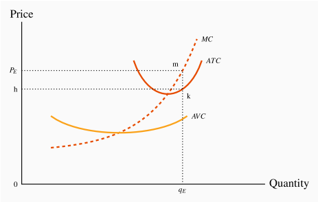
Let us return to our graphical analysis, and begin by supposing that the market equilibrium described in Figure 9.4 results in profits being made by some firms. Such an outcome is described in Figure 9.5, where the price exceeds the ATC. At the price  , a profit-making firm supplies the quantity
  , as determined by its MC curve. On average, the cost of producing each unit of output, , is defined by the point on the ATC at that output level, point k. Profit per unit is thus given by the value (m–k) – the difference between revenue per unit and cost per unit. Total (economic) profit is therefore the area
  , which is quantity times profit per unit.
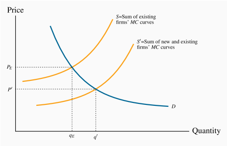
While represents an equilibrium for the firm, it is only a short-run, or temporary, equilibrium for the industry. The assumption of free entry and exit implies that the presence of economic profits will induce new entrepreneurs to enter and start producing. The impact of this dynamic is illustrated in Figure 9.6. An increased number of firms shifts supply rightwards to become  , thereby increasing the amount supplied at any price. The impact on price of this supply shift is evident: With an unchanged demand, the equilibrium price must fall.
How far will the price fall, and how many new firms will enter this profitable industry? As long as economic profits exist new firms will enter and the resulting increase in supply will continue to drive the price downwards. But, once the price has been driven down to the minimum of the ATC of a representative firm, there is no longer an incentive for new entrepreneurs to enter. Therefore, the long-run industry equilibrium is where the market price equals the minimum point of a firm's ATC curve. This generates normal profits, and there is no incentive for firms to enter or exit.
A long-run equilibrium in a competitive industry requires a price equal to the minimum point of a firm's ATC. At this point, only normal profits exist, and there is no incentive for firms to enter or exit.
In developing this dynamic, we began with a situation in which economic profits were present. However, we could have equally started from a position of losses. With a market price between the minimum of the AVC and the minimum of the ATC in Figure 9.5, revenues per unit would exceed variable costs but not total costs per unit. When firms cannot cover their ATC in the long run, they will cease production. Such closures must reduce aggregate supply; consequently the market supply curve contracts, rather than expands as it did in Figure 9.6. The reduced supply drives up the price of the good. This process continues as long as firms are making losses. A final industry equilibrium is attained only when the price reaches a level where firms can make a normal profit. Again, this will be at the minimum of the typical firm's ATC.
Accordingly, the long-run equilibrium is the same, regardless of whether we begin from a position in which firms are incurring losses, or where they are making profits.
Application Box 9.2 Entry and exit: Oil rigs
Oil drilling is a competitive market. There are a large number of suppliers, information is ubiquitous, and entry and exit are relatively free.
In the years 2012 and 2013 the price of crude oil was around $100 US per barrel. Towards the end of 2014 the price of oil began to drop on world markets, and by early 2015 it fluctuated around $50. The response of drillers in the US was substantial and immediate. The number of active rigs declined dramatically. In terms of our economic model, certain suppliers exited; they moth-balled their rigs and waited for the price of oil to recover.
Another such cycle, even more pronounced, occurred in 2020. With the coronavirus pandemic, the demand for oil dropped and its price plummeted. Again, many firms shut down their rigs and had no choice but to sit out the price decline. A highly informative graphic is presented at https://tradingeconomics.com/united-states/crude-oil-rigs.
In addition to the decline in traditional oil recovery rigs, the number of operating shale crews declined by even greater amounts. Details at https://www.forbes.com/sites/davidblackmon/2020/05/12/a-grim-earnings-season-for-the-us-shale-business/#6f55a95a1cf2