9.5: Long-run industry supply

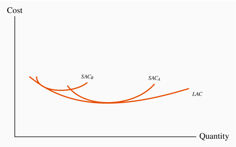
When aggregating the firm-level supply curves, as illustrated in Figure 9.3, we did not assume that all firms were identical. In that example, firm A has a cost structure with a lower AVC curve, since its supply curve starts at a lower dollar value. This indicates that firm A may have a larger plant size than firm B – one that puts A closer to the minimum efficient scale region of its long-run ATC curve.

Figure 9.7 Firms with different plant sizes

Firm B cannot compete with Firm A in the long run given that B has a less efficient plant size than firm A. The equilibrium long-run price equals the minimum of the LAC. At this price firm B must move to a more efficient plant size or make losses.

Can firm B survive with his current scale of operation in the long run? Our industry dynamics indicate that it cannot. The reason is that, provided some firms are making economic profits, new entrepreneurs will enter the industry and drive the price down to the minimum of the ATC curve of those firms who are operating with the lowest cost plant size. B-type firms will therefore be forced either to leave the industry or to adjust to the least-cost plant size—corresponding to the lowest point on its long-run ATC curve. Remember that the same technology is available to all firms; they each have the same long-run ATC curve, and may choose different scales of operation in the short run, as illustrated in Figure 9.7. But in the long run they must all produce using the minimum-cost plant size, or else they will be driven from the market.

This behaviour enables us to define a long-run industry supply. The long run involves the entry and exit of firms, and leads to a price corresponding to the minimum of the long-run ATC curve. Therefore, if the long-run equilibrium price corresponds to this minimum, the long-run supply curve of the industry is defined by a particular price value—it is horizontal at the price corresponding to the minimum of the LATC. More or less output is produced as a result of firms entering or leaving the industry, with those present always producing at the same unit cost in a long-run equilibrium.

Industry supply in the long run in perfect competition is horizontal at a price corresponding to the minimum of the representative firm's long-run ATC curve.

Figure 9.8 Long-run dynamics

The LR equilibrium price P_E is disturbed by a shift in demand from D₁ to D₂. With a fixed number of firms, P₂ results. Profits accrue at this price and entry occurs. Therefore the SR supply shifts outwards until these profits are eroded and the new equilibrium output is Q₂. If, instead, D falls to D₃ then firms exit because they make losses, S shifts back until the price is driven up sufficiently to restore normal profits. Different outputs are supplied in the long run at the same price P_E, therefore the long-run supply is horizontal at P_E.

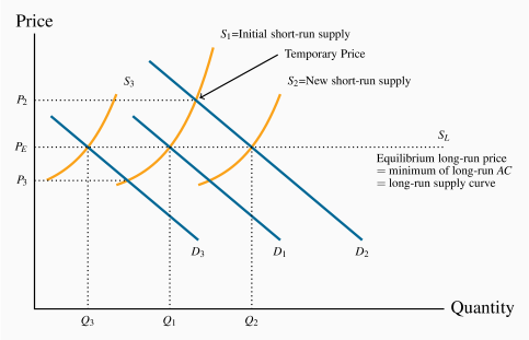
This industry's long-run supply curve, S_L, and a particular short-run supply are illustrated in Figure 9.8. Different points on S_L are attained when demand shifts. Suppose that, from an initial equilibrium Q₁, defined by the intersection of D₁ and S₁, demand increases from D₁ to D₂ because of a growth in income. With a fixed number of firms, the additional demand can be met only at a higher price (P₂), where each existing firm produces more using their existing plant size. The economic profits that result induce new operators to produce. This addition to the industry's production capacity shifts the short-run supply outwards and price declines until normal profits are once again being made. The new long-run equilibrium is at Q₂, with more firms each producing at the minimum of their long-run ATC curve, P_E.

The same dynamic would describe the industry reaction to a decline in demand—price would fall, some firms would exit, and the resulting contraction in supply would force the price back up to the long-run equilibrium level. This is illustrated by a decline in demand from D₁ to D₃.

Increasing and decreasing cost industries

While a horizontal long-run supply is the norm for perfect competition, in some industries costs increase with the scale of industry output; in others they decrease. This may be because all of the producers use a particular input that itself becomes more or less costly, depending upon the amount supplied.

Figure 9.9 Increasing and decreasing cost industries

When individual-supplier costs rise as the output of the industry increases we have an increasing cost supply curve for the industry in the long run. Conversely, when the costs of individual suppliers fall with the scale of the industry, we have a decreasing cost industry.

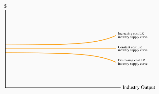
Decreasing cost sectors are those that benefit from a decline in the prices of their inputs as the size of their market expands. This is frequently because the suppliers of the inputs themselves can benefit from scale economies as a result of expansion in the market for the final good. A case in point has been the computer market, or the tablet market: As output in these markets has grown, the producers of videocards and random-access memory have benefited from scale economies and thus been able to sell these components at a lower price to the manufacturers of the final goods. An example of an increasing cost market is the market for landings and take-offs at airports. Airports are frequently limited in their ability to expand their size and build additional runways. In such markets, as use grows, planes about to land may have to adopt a circling holding pattern, while those departing encounter clearance delays. Such delays increase the time costs to passengers and the fuel and labour costs to the suppliers. Decreasing and increasing industry costs are reflected in the long-run industry supply curve by a downward-sloping segment or an upward sloping segment, as illustrated in Figure 9.9.

Increasing (decreasing) cost industry is one where costs rise (fall) for each firm because of the scale of industry operation.