The value of labour springs from the value of its use, that is the value placed upon goods and services that it produces – product prices. The wage is the price that equilibrates the supply and demand for a given type of labour, and it reflects the value of that labour in production. Formally, the demand for labour (and capital) is thus a derived demand, in contrast to being a 'final' demand.
Demand for labour: a derived demand, reflecting the value of the output it produces.
We must distinguish between the long run and the short run in our analysis of factor markets. On the supply side certain factors of production are fixed in the short run. For example, the supply of radiologists can be increased only over a period of years. While one hospital may be able to attract radiologists from another hospital to meet a shortage, this does not increase the supply in the economy as a whole.
On the demand side there is the conventional difference between the short and long run: In the short run some of a firm's factors of production, such as capital, are fixed, and therefore the demand for labour differs from when all factors are variable – the long run.
Demand in the short run
Table 12.1 contains information from the example developed in Chapter 8. It can be used to illustrate how a firm reacts in the short run to a change in an input price, or to a change in the output price. The response of a producer to a change in the wage rate constitutes a demand function for labour – a schedule relating the quantity of the input demanded to different input prices. The output produced by the various numbers of workers yields a marginal product curve, whose values are stated in column 3. The marginal product of labour,  , as developed in Chapter 8, is the additional output resulting from one more worker being employed, while holding constant the other (fixed) factors. But what is the dollar value to the firm of an additional worker? It is the additional value of output resulting from the additional employee – the price of the output times the worker's marginal contribution to output, his MP. We term this the value of the marginal product.
The value of the marginal product is the marginal product multiplied by the price of the good produced.
Table 12.1 Short-run production and labour demand
| Workers |
Output |
MPL |
 |
Marginal profit = (VMPL–wage) |
| (1) |
(2) |
(3) |
(4) |
(5) |
| 0 |
0 |
|
|
|
| 1 |
15 |
15 |
1050 |
150 |
| 2 |
40 |
25 |
1750 |
750 |
| 3 |
70 |
30 |
2100 |
1100 |
| 4 |
110 |
40 |
2800 |
1800 |
| 5 |
145 |
35 |
2450 |
1450 |
| 6 |
175 |
30 |
2100 |
1100 |
| 7 |
200 |
25 |
1750 |
750 |
| 8 |
220 |
20 |
1400 |
400 |
| 9 |
235 |
15 |
1050 |
50 |
| 10 |
240 |
5 |
350 |
negative |
Each unit of labour costs $1,000; output sells at a fixed price of $70 per unit.
In this example the first rises as more labour is employed, and then falls. With each unit of output selling for $70 the value of the marginal product of labour ( ) is given in column 4. The first worker produces 15 units each week, and since each unit sells for a price of $70, his production value to the firm is $1,050
  . A second worker produces 25 units, so his value to the firm is $1,750, and so forth. If the weekly wage of each worker is $1,000 then the firm can estimate its marginal profit from hiring each additional worker. This is the difference between the value of the marginal product and the wage paid, and is given in the final column of the table.
It is profitable to hire more workers as long as the cost of an extra worker is less than the . The equilibrium amount of labour to employ is therefore 9 units in this example. If the firm were to hire one more worker the contribution of that worker to its profit would be negative  , and if it hired one worker less it would forego the opportunity to make an additional profit of $50 on the 9th unit
  .
.
Profit maximizing hiring rule:
- If the VMPL of next worker > wage, hire more labour.
- If the VMPL < wage, hire less labour.
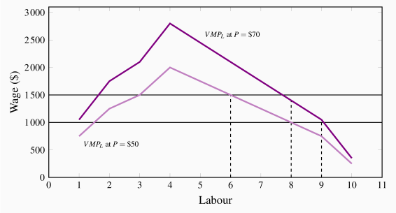
To this point we have determined the profit maximizing amount of labour to employ when the output price and the wage are given. However, a demand function for labour reflects the demand for labour at many different wage rates, just as the demand function for any product reflects the quantity demanded at various prices. Accordingly, suppose the wage rate is $1,500 per week rather than $1,000. The optimal amount of labour to employ in this case is determined in exactly the same manner: Employ the amount of labour where its contribution is marginally profitable. Clearly the optimal amount to employ is 7 units: The value of the seventh worker to the firm is $1,750 and the value of the eighth worker is $1,400. Hence it would not be profitable to employ the eighth, because his marginal contribution to profit would be negative. Following the same procedure we could determine the optimal amount of labour to employ at different wages. This implies that the function is the demand for labour function because it determines the most profitable amount of labour to employ at any wage.
The optimal amount of labour to hire is illustrated in Figure 12.1. The wage and VMPL curves come from Table 12.1. The VMPL curve has an upward sloping segment, reflecting increasing productivity, and then a regular downward slope as developed in Chapter 8. At employment levels where the VMPL is greater than the wage additional labour should be employed. But when the VMPL falls below the wage rate employment should stop. If labour is divisible into very small units, the optimal employment decision is where the MPL function intersects the wage line.
Figure 12.1 also illustrates what happens to hiring when the output price changes. Consider a reduction in its price to $50 from $70. The profit impact of such a change is negative because the value of each worker's output has declined. Accordingly, the demand curve must reflect this by shifting inward (down), as in the figure. At various wage rates, less labour is now demanded. The new schedule can be derived in Table 12.1 as before: It is the schedule multiplied by the lower value ($50) of the final good.
In this example the firm is a perfect competitor in the output market, because the price of the good it produces is fixed. It can produce and sell more of the good without this having an impact on the price of the good in the marketplace. Where the firm is not a perfect competitor it faces a declining MR function. In this case the value of the is the product of MR and rather than P and . To distinguish the different output markets we use the term marginal revenue product of labour ( ) when the demand for the output slopes downward. But the optimizing principle remains the same: The firm should calculate the value of each additional unit of labour, and hire up to the point where the additional revenue produced by the worker exceeds or equals the additional cost of that worker.
The marginal revenue product of labour is the additional revenue generated by hiring one more unit of labour where the marginal revenue declines.
Demand in the long run
In Chapter 8 we proposed that firms choose their factors of production in accordance with cost-minimizing principles. In producing a specific output, firms choose the least-cost combination of labour and plant size. But how is this choice affected when the price of labour or capital changes? While adjustment to price changes may require a long period of time, we know that if one factor becomes more (less) expensive, the firm will likely change the mix of capital and labour away from (towards) that factor. For example, when the accuracy and prices of production robots began to fall in the nineteen nineties, auto assemblers reduced their labour and used robots instead. When computers and computer software improved and declined in price, clerical workers were replaced by computers that were operated by accountants. But such adjustments and responses do not occur overnight.
In the short run a higher wage increases costs, but the firm is constrained in its choice of inputs by a fixed plant size. In the long run, a wage increase will induce the firm to use relatively more capital than when labour was less expensive in producing a given output. But despite the new choice of inputs, a rise in the cost of any input must increase the total cost of producing any output.
A change in the price of any factor has two impacts on firms: In the first place producers will substitute away from the factor whose price increases; second, there will be an impact on output and a change in the price of the final good it produces. Since the cost structure increases when the price of an input rises, the supply curve in the market for the good must reflect this – any given output will now be supplied at a higher price. With a downward sloping demand, this shift in supply must increase the price of the good and reduce the amount sold. This second effect can be called an output effect.
Monopsony
Some firms may have to pay a higher wage in order to employ more workers. Think of Hydro Quebec building a dam in Northern Quebec. Not every hydraulic engineer would be equally happy working there as in Montreal. Some engineers may demand only a small wage premium to work in the North, but others will demand a high premium. If so, Hydro Quebec must pay a higher wage to attract more workers – it faces an upward sloping supply of labour curve. Hydro Quebec is the sole buyer in this particular market and is called a monopsonist – a single buyer. Our general optimizing principle governing the employment of labour still holds, even if we have different names for the various functions: Hire any factor of production up to the point where the cost of an additional unit equals the value generated for the firm by that extra worker. The essential difference here is that when a firm faces an upward sloping labour supply it will have to pay more to attract additional workers and also pay more to its existing workers. This will impact the firm's willingness to hire additional workers.
A monopsonist is the sole buyer of a good or service and faces an upward-sloping supply curve.
Application Box 12.1 Monopsonies
Monopsonies are more than a curiosity; they exist in the real world. An excellent example is the cannabis market in Canada. Virtually every province has set up a trading agency that has the sole right to purchase cannabis from growers; growers and processors are not permitted to sell directly to retailers; they may only sell to the monopsony by law. In turn, these provincial cannabis monopsonies are frequently retail monopolists in that the agency owns all of the retail outlets in the province.
Firm versus industry demand
The demand for labour within an industry, or sector of the economy, is obtained from the sum of the demands by each individual firm. It is analogous to the goods market, but with a subtle difference. In Chapter 3 we obtained a market demand by summing individual demands horizontally. The same could be done here: At lower (or higher) wages, each firm will demand more (or less) labour. However, if all firms employ more labour in order to increase their output, the price of the output will likely decline. This in turn will moderate the demand for labour – it is slightly less valuable now that the price of the output it produces has fallen. This is a subtle point, and we can reasonably think of the demand for labour in a given sector of the economy as the sum of the demands on the part of the employers in that sector.