Explore the components of the federal budget and the federal debt
Analyze the macroeconomic impact of expansionary and contractionary fiscal policy
Examine the macroeconomic impact of government budget deficits and surpluses
Distinguish between marginal tax rates and average tax rates in different taxation systems
Develop the concept of a tax rate multiplier
Investigate the implications of fiscal policy for macroeconomic stability
Demonstrate the value of a concept referred to as the full employment budget
Contrast Keynesian full employment policies with neoclassical austerity policies
Evaluate a Marxian theory of government borrowing and debt
In Chapter 17, we investigated the role of the central bank and how monetary policy may be used to influence aggregate output, employment, and the general price level from several different theoretical perspectives. In this chapter, we consider the role of the federal government and how fiscal policy may be used to influence key macroeconomic variables from different vantage points, including neoclassical, Keynesian, and Marxian perspectives. To set the stage, we will define such concepts as government deficits and government debt and then look at the structure of the federal budget for Fiscal Year 2015. Next, we will investigate the macroeconomic impacts of expansionary and contractionary fiscal policy and government deficits and surpluses from neoclassical and Keynesian perspectives. We will then look at different systems of taxation and how to develop a tax rate multiplier to be used in the Keynesian Cross model. Additional topics include the implications of fiscal policy for macroeconomic stability, the usefulness of the concept of the full employment budget, and the contrast between Keynesian full employment policies and neoclassical austerity policies. We will conclude with a Marxian analysis of government borrowing and government debt.
The Federal Budget and the FederalDebt
Fiscal policy pertains to the use of government spending and taxation to influence aggregate output, employment and the price level. The federal government spends a great deal of money, but it also receives a great deal of money through tax collections and other sources. When government outlays and receipts for the year do not match, we say that the budget is out of balance. When government outlays and government receipts for the year do match, then we refer to a balanced budget. When government outlays exceed government receipts for the year, then we say that a budget deficit exists. Finally, when government outlays fall short of government receipts for the year, then we say that a budget surplus exists. Using R to represent government receipts and O to represent government outlays, we can list the possibilities as follows:
Although we speak in terms of an annual budget, it is not the calendar year that we have in mind but rather the government’s fiscal year, which begins on October 1 of each year and ends the following September 30. For example, Fiscal Year 2018 (FY2018) includes the date October 5, 2017 but not September 25, 2017.
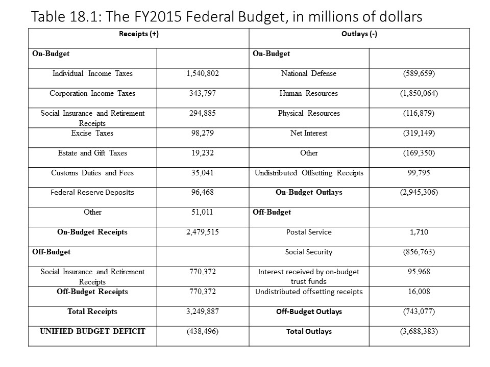
To develop a sense of which items the federal budget includes, let’s consider the figures for FY2015. Table 18.1 shows the Unified Federal Budget for FY2015, which lists all Federal outlays and receipts for that year.[1]
Only some items have been listed in Table 18.1 with the remaining items included in “Other” categories. Also, the receipts and outlays have been divided according to whether they are “on-budget” or “off-budget.” The federal government’s unified budget includes all receipts and outlays of the federal government. Some receipts and outlays, however, are treated as off-budget because of a desire to protect them from lawmakers, in the case of Social Security, for example, or because it is viewed as a part of the budget that should be able to achieve balance independently, as in the case of the U.S. Postal Service.
To calculate the unified budget deficit or unified budget surplus, we simply add up the total receipts and subtract the total outlays to obtain a unified budget deficit of $438.496 billion. It is also possible to calculate the on-budget deficit or on-budget surplus and the off-budget deficit or off-budget surplus. In the former case, we take the on-budget receipts and subtract the on-budget outlays to obtain an on-budget deficit of $465.791 billion. In the latter case, we take the off-budget receipts and subtract the off-budget outlays to obtain an off-budget surplus of $27.295 billion.
The on-budget deficit and the off-budget surplus may be added together to obtain the unified budget deficit. To understand why, consider the following equation:
In the above equation, the sum of on-budget receipts (RN) and off-budget receipts (RF) is calculated and then we subtract the sum of on-budget outlays (ON) and off-budget outlays (OF). Rearranging the terms, we obtain the following result:
That is, we can simply sum together the on-budget balance and the off-budget balance to obtain the unified budget balance. In this example, if we add the off-budget surplus to the on-budget deficit, then we obtain the unified budget deficit of $438.496 billion. This example demonstrates the benefit of reporting the off-budget balance separately from the on-budget balance. Because the Social Security program has had many years of surpluses, its inclusion in the unified budget has made the federal deficit appear smaller than it is. If we focus on the part of the budget over which lawmakers have more control from year to year (i.e., the on-budget deficit), then we can see that the federal deficit was somewhat larger in FY2015 and has been far larger than the unified budget deficit in some years due to large Social Security surpluses.
The complete federal budget contains many items, but federal outlays can be divided into three major categories. Frequently, the appropriated programs or discretionary programs are grouped together because they require Congress to pass annual appropriations bills. These outlays include spending on agriculture, defense, education, energy, homeland security, health and human services, housing and urban development, environmental protection, and so on. Mandatory spending, on other hand, includes entitlement programs that do not depend on Congress to pass annual appropriations bills and where the outlays depend on who qualifies for benefits under federal law. Examples include Social Security, Medicare, and Medicaid. The final major component is net interest, which accounts for interest paid to owners of U.S. government bonds less the interest that the government receives. The total outlays for FY2015 amounted to $3,688.383 billion, or $3.688383 trillion, as shown in Table 18.1.
Federal receipts for FY2015 include several different sources, including individual income taxes, corporate income taxes, Social Security payroll taxes, Medicare payroll taxes, unemployment insurance taxes, excise taxes, estate and gift taxes, customs duties, and profit distributions from the Federal Reserve. The total receipts for FY2015 amounted to $3,249.887 billion, or $3.249887 trillion, as shown in Table 18.1.
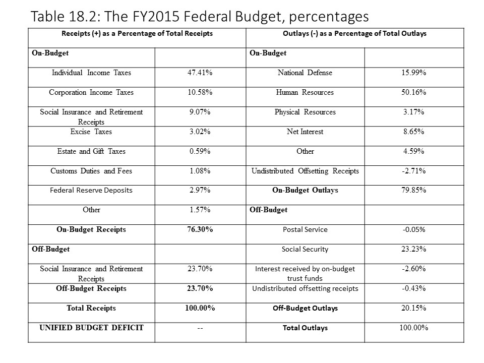
Table 18.2 shows federal receipts and federal outlays as percentages of their totals for FY2015.[2]
The percentages reveal which items represent the largest shares of the total receipts and total outlays. In terms of receipts, individual incomes taxes represent the largest share, followed by Social Security receipts and corporate income taxes. In terms of outlays, Human Resources, Social Security, and National Defense represent the largest shares, followed by net interest payments on the debt.
The federaldebt represents the entire accumulated debt of the federal government minus whatever has been repaid over the years. In any given year, when federal receipts fall short of federal outlays, it is necessary for the federal government to borrow to make up the difference. These borrowings add to the federal debt. Therefore, the federal debt may be thought of as the accumulation of past federal deficits (less any repayments out of federal surpluses). Deficits and surpluses, therefore, represent flow variables because they are measured on an annual basis. The national debt, on the other hand, represents a stock variable because we can identify the total amount owed at a given point in time.
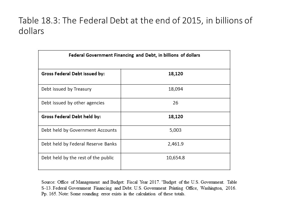
At the end of FY2015, total gross federal debt amounted to $18.120 trillion. Most of the borrowed funds (about $18.094 trillion) was acquired through the issuance and sale of Treasury securities. The remainder (about $26 billion) was acquired via the issuance and sale of federal agency bonds. This information is presented in Table 18.3.
The buyers of these government bonds are the holders of U.S. government debt obligations. These bonds represent promises of the U.S. government to repay the face values and to maintain regular interest payments until the bonds mature. Who owns these bonds? Interestingly, a large portion of these bonds (about $5.003 trillion) is held in U.S. Government accounts such as the Social Security Trust Fund. When the Social Security program has a surplus, for example, this amount is invested in a special category of U.S. Treasury bonds. The Federal Reserve Banks hold another portion of the debt (about $2.4619 trillion). The remaining $10.6548 trillion is held by the rest of the public. It is surprising to many people that such a large percentage of the federal debt (about 41.2%) is owed to the federal government or to the nation’s quasi-public central bank.
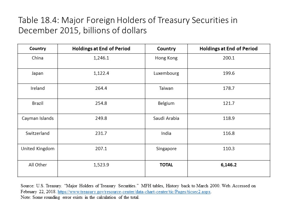
Domestic and foreign investors own the part of the debt that the federal government and the Fed do not own. At the end of December 2015, the total foreign holdings of Treasury securities amounted to $6,146.2 billion, or $6.1462 trillion. China and Japan are the largest holders of U.S. Treasury securities with more than $1.1 trillion each in FY2015. All foreign nations with more than $100 billion of Treasury securities in FY2015 are listed in Table 18.4.
The foreign holdings of Treasury securities amount to approximately 1/3 of the federal debt. These basic facts about the federal budget and the federal debt will be useful as we consider the macroeconomic impacts of each from a variety of perspectives.
Expansionary Fiscal Policy versus Contractionary Fiscal Policy
The federal government may use fiscal policy to pursue an economic expansion. In that case, it implements an expansionary fiscal policy with the aim of promoting higher aggregate output and employment. On the other hand, the federal government might use fiscal policy to restrict the growth of output and employment. The government is then said to be implementing a contractionary fiscal policy, which it might implement due to its fear of inflation.
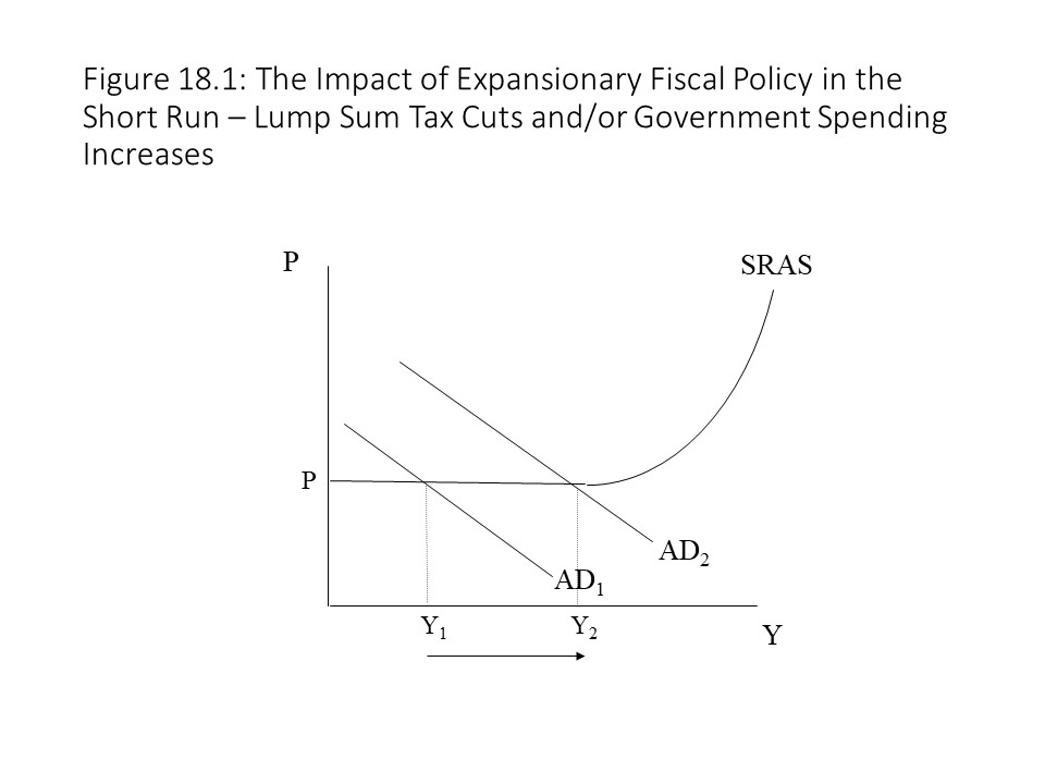
Expansionary fiscal policy might be implemented in several different ways. To pursue an economic expansion, the federal government might cut taxes, increase government spending, or combine the two policies.[3] Each measure will stimulate aggregate demand, and if implemented in the short run when prices are sticky, the rise in aggregate demand will increase real output and employment as shown in Figure 18.1.
The precise impact on real output, however, depends on the size of the lump sum tax multiplier and the government expenditures multiplier.
The reader should recall that the lump sum tax multiplier is the following:
Similarly, the government expenditures multiplier is the following:
Suppose that the government cuts taxes by $50 billion, and the marginal propensity to consume (mpc) is 3/4. Then the lump sum tax multiplier is equal to -3 and we can calculate the change in real output as follows:
That is, a tax cut of $50 billion increases real output by $150 billion. The reason for the multiplier is that households have more after-tax income to spend, which triggers additional rounds of household spending. Ultimately, real output increases three times as much as the tax cut.
Now suppose that the government increases spending by $50 billion, and the mpc is ¾. The government expenditures multiplier in this case is equal to 4, and we can calculate the change in real output as follows:
A government spending increase of $50 billion increases real output by $200 billion. The reason for the multiplier is that households receive the government spending as income and then spend it, which triggers even more consumption. In the end, real output rises by four times the initial increase in spending.
Finally, consider a combination of government spending increases and tax cuts, not unlike the policy pursued in early 2009 when Congress passed the American Recovery Act. This piece of legislation included a mix of tax cuts and spending increases aimed at boosting economic activity during the Great Recession. Suppose that the government increases spending by $20 billion and cuts taxes by $40 billion. Continue to assume that the mpc is ¾. In this case, real output receives a boost from both sources as follows:
This example shows that a combination of a tax cut and a smaller spending increase can achieve the same increase in real output as the larger spending increase. In all three cases, aggregate demand experiences a rightward shift, and real output and employment expand as a result.
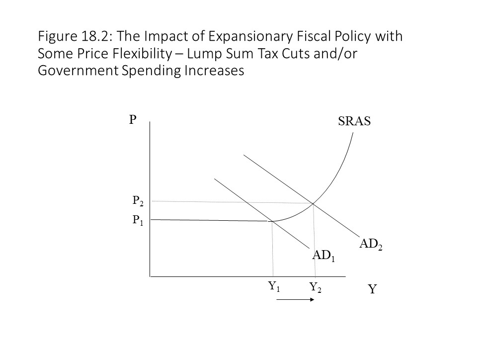
It is also worth noting that the full multiplier effects are felt only if prices are sticky in the short run as shown in Figure 18.1. The situation is somewhat different if prices are at least partly flexible as shown in Figure 18.2.
In Figure 18.2, the rise in real output is somewhat offset due to the rising price level. As the economy approaches the full employment level of real output, some of the aggregate demand increase leads to higher prices in addition to higher real output. Since the full impact of the rise in aggregate demand is not felt on real output, the multipliers do not fully function. In the extreme case where AD rises and intersects the vertical portion of the AS curve, prices are completely flexible and the multipliers are not operative at all with real output stuck at the full employment level. The case of perfect price flexibility is the neoclassical assumption whereas the assumption of sticky prices is the Keynesian assumption.
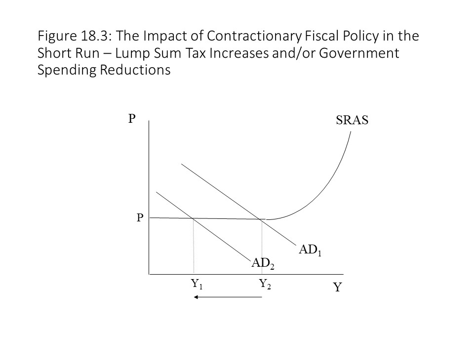
Contractionary fiscal policy might also be implemented in several different ways. To pursue an economic contraction, the federal government might raise taxes, cut government spending, or combine the two policies. Each measure will reduce aggregate demand, and if implemented in the short run when prices are sticky, the drop in aggregate demand will decrease real output and employment as shown in Figure 18.3.
As before, the precise impact on real output depends on the size of the lump sum tax multiplier and the government expenditures multiplier.
Suppose that the government raises taxes by $50 billion, and the mpc is 3/4. Then the lump sum tax multiplier is equal to -3 and we can calculate the change in real output as follows:
That is, a tax increase of $50 billion reduces real output by $150 billion. The reason for the multiplier effect here is that households have less after-tax income to spend, which triggers additional reductions of household spending. Ultimately, real output falls three times as much as the tax increase.
Now suppose that the government reduces spending by $50 billion, and the mpc is ¾. The government expenditures multiplier in this case is equal to 4, and we can calculate the change in real output as follows:
A government spending reduction of $50 billion decreases real output by $200 billion. The reason for the multiplier effect in this case is that households no longer receive the government spending as income and so cannot spend it, which triggers even less consumption. In the end, real output falls by four times the initial reduction in spending.
Finally, consider a combination of government spending reductions and tax increases. Suppose that the government reduces spending by $20 billion and raises taxes by $40 billion. In this case, real output receives a boost from both sources as follows:
This example shows that a combination of a tax increase and a smaller spending reduction can achieve the same decrease in real output as the larger spending reduction. In all three cases, aggregate demand experiences a leftward shift and real output and employment contract as a result. The benefit to the economy is that less danger exists that a sudden rise in aggregate demand will lead to inflation.
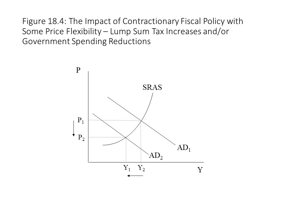
It is also worth noting that the full multiplier effects are felt only if prices are sticky in the short run and downwardly inflexible as shown in Figure 18.3. The situation is somewhat different if prices are at least partly flexible as shown in Figure 18.4.
In Figure 18.4, the fall in real output is somewhat offset due to the falling price level. As the economy contracts, some of the aggregate demand reduction leads to lower prices in addition to lower real output. Since the full impact of the fall in aggregate demand is not felt on real output, the multipliers do not fully function, and deflation occurs. In the extreme case where AD falls and intersects the vertical portion of the AS curve, prices are completely flexible and the multipliers are not operative at all with real output stuck at the full employment level even as AD and the price level fall.
The Macroeconomic Impacts of Government Budget Deficits and Surpluses
When the federal government runs a budget deficit, it typically borrows to make up the difference. Printing the money is another option, but modern economies have rejected this solution given its tendency to produce hyperinflation. When a government wishes to borrow to cover its budget deficit, it must issue bonds and sell them to the public. This entrance into the loanable funds market and the bond market has the potential to alter interest rates and bond prices, which then carries consequences for the rest of the economy.
Suppose the government is borrowing in the loanable funds market, which permits it to run a budget deficit. At the same time, assume that the central bank is tightly controlling the supply of loanable funds such that it always adjusts the supply of loanable funds to offset any change in the equilibrium quantity exchanged in this market. The increased government borrowing will raise the demand for loanable funds, which creates a shortage and drives up the interest rate. The equilibrium quantity exchanged rises too. Because the central bank is regulating the quantity of loanable funds, it reduces the supply of loanable funds using its monetary policy tools. These changes to the supply and demand for loanable funds are shown in Figure 18.5.
The reduction in the supply of loanable funds causes a leftward shift of the supply curve, which drives the interest rate up further but causes the equilibrium quantity exchanged to return to its original level. The refusal of the central bank to accommodate the increase in government borrowing has led to a higher interest rate, which completely crowds out debt-financed private investment and consumption. That is, government spending on goods and services expands entirely at the expense of private sector spending on goods and services. In terms of the AD/AS model, the increase in debt-financed government spending will increase aggregate demand, but the higher interest rates reduce investment spending and consumer spending, which leaves AD unchanged in the end as shown in Figure 18.5. In this scenario involving complete crowding out of private investment, the composition of total output changes with a shift away from investment spending and towards government spending, but the aggregate output is not affected.[4] It is also worth noting that the multiplier effect is completely inoperative in this situation even though the price level is constant.Figure 18.6.The increased demand for loanable funds in Figure 18.6 causes the interest rate and the quantity exchanged to increase. Although the interest rate rises, it does not rise as much as it does when the central bank also restricts the supply of loanable funds. This scenario involves the partial crowding out of private investment spending and private consumer spending because the higher demand does manage to increase the equilibrium quantity in this market even as the interest rate rises. The partial crowding out is reflected in the movement along the new demand curve as the interest rate rises. In this case, the increase in government spending shifts the AD curve to the right, which then partially shifts back to the left due to the reduction in consumer spending and investment spending as the interest rate rises. The multiplier effect is lessened in this situation as well due to the rise in interest rates even though the price level is constant.Figure 18.7.In Figure 18.7 the demand for loanable funds increases due to government borrowing, but then the supply of loanable funds also rises as the central bank accommodates the increased demand for loans. The rightward shift of the demand curve raises the equilibrium quantity and the interest rate. The rightward shift of the supply further raises the equilibrium quantity but brings the interest rate back down to the original level. Because the interest rate does not change in this situation, no crowding out of private investment or private consumption occurs, and the full multiplier effect is operative if the price level is constant. This scenario was discussed in Chapter 17 in the context of Post-Keynesian endogenous money supply theory. The Fed accommodates the higher demand for loanable funds with an increase in the money supply. If prices are sticky, then the full impact of the higher money supply is felt on real output. If the rightward shift of AD occurred in the upward sloping portion of the SRAS curve, then the rise in the price level would lessen the impact on real output. Even with a rise in the price level, however, no crowding out occurs because the interest rate does not rise.Figure 18.8.When the dollar appreciates, U.S. exports become more expensive for foreign buyers and imports become cheaper for American buyers. The consequence is a reduction in U.S. exports and a rise in U.S. imports. Net exports thus fall, which causes a leftward shift of the AD curve, partially offsetting the rightward shift of AD due to higher government spending.Figure 18.9.If the exchange rate returns to its original level, then net exports should not be negatively affected even though the government deficit spending will still lead to a rise in interest rates and partial crowding out. The partial crowding out in this case would involve a leftward shift of AD from AD2 (not shown in the graph), but the shift would not be as large as that shown in Figure 18.8 because a reduction in net exports does not contribute to the decline in aggregate demand in this case.Figure 18.10.
The consequence of the central bank’s supply reduction is a further appreciation of the U.S. dollar even as it stabilizes the quantity exchanged of dollars. Figure 18.10 assumes that the crowding out of private investment and the negative impact on net exports exactly offset the expansionary impact of the deficit spending. The impact on U.S. net exports could be so extreme, however, that combined with the partial crowding out of private investment, the consequent drop in real output and employment could more than cancel the expansionary impact of the government deficit spending.
The examples in this section demonstrate that expansionary fiscal policy may be partly offset, completely offset, or not at all offset by action that the central bank takes. Coordination among policymakers is essential so that fiscal policy and monetary policy do not work against one another in terms of their impact on output, employment, and the price level.
A very different possibility is that the federal government manages to run a budget surplus. In that situation, it must decide how to use the surplus, and the repayment of federal debt is one possibility. If the government chooses this option, then it repays the bondholders. The bondholders then possess loanable funds that they will probably wish to lend again. The likely result then is an increase in the supply of loanable funds as shown in Figure 18.11.
In this example, the increased supply creates a surplus of loanable funds and pushes the rate of interest down. The drop in the rate of interest stimulates investment spending and consumer spending. Aggregate demand thus shifts to the right. If prices are sticky, the impact is an unambiguous gain for the economy with rising real output and employment and a stable price level. If the economy is close to full employment, however, the risk of the rise in the supply of loanable funds is demand-pull inflation.[5]
Marginal Tax Rates and Average Tax Rates
Up to this point, it has been assumed that the government simply appropriates tax revenue in one lump sum amount from the households each year. The lump sum tax (T) is not very realistic because households are taxed a specific percentage of their incomes. In fact, different tax rates apply to different income levels. For example, in 2017 a single taxpayer paid 10% of the first $9,325 of income in taxes to the federal government. For earnings between $9,325 and $37,950, a single taxpayer paid a 15% tax rate while still paying a 10% tax rate on the first $9,325 earned. The tax rates that apply to different income tax brackets are called marginal tax rates. Marginal tax rates tell us how much of an additional dollar of income is paid in taxes. Income tax brackets tell us the range of income to which a specific marginal tax rate applies. Table 18.5 shows the marginal tax rates and income tax brackets for a single taxpayer filing in 2017.
Table 18.5 also shows us how much tax is paid if one earns the median income in each tax bracket. The median income is the income level that is exactly halfway between the highest and lowest income levels in the tax bracket. For example, the median income levels in the 10% and 15% income tax brackets are equal to $4,662.50 and $23,637.50, respectively, and are calculated as follows:
To determine the taxes owed on the median income in any tax bracket, we cannot simply multiply that median income level by the marginal tax rate that applies to that tax bracket. To calculate the taxes owed in this manner would assume that a single tax rate applies to the entire income. The correct calculation requires that we multiply each increment of income up to that income level by the appropriate marginal income tax rate. For example, to calculate the taxes owed for someone who earns $141,775 (the median income in the 28% income tax bracket), we do the following:
The taxes owed for other income levels are determined in a similar fashion. It is simple to determine the percentage of income that is owed in taxes, which is called the average tax rate. To calculate the average tax rate, simply divide the total taxes owed by the income level as follows:
For example, the median income level in the 33% income tax bracket is $304,175, and the taxes owed are $83,777. The average tax rate is calculated as follows:
The reader should notice that the marginal income tax rates increase with income level. As a result, the taxes owed rise more quickly than income as income increases. The result is a rising average tax rate, which is also visible in the table. When the average tax rate increases with income, the system of taxation is referred to as a progressive tax system. When a person earns more income in such a tax system, the total taxes owed increase but also the percentage of income paid in taxes increases. The justification for a tax system of this kind is that it makes possible the government redistribution of income and thus has the potential to reduce after-tax income inequality.
Those who oppose progressive taxation systems frequently advocate a single marginal tax rate that applies to all levels of income. In this case, the taxes owed and the income level rise at the same rate, which leaves the average tax rate unchanged. When the average tax rate remains constant at all levels of income, the system of taxation is referred to as a proportional tax system. A proportional tax is more commonly called a flat tax.
A third type of taxation system involves marginal tax rates that decrease as the income level rises. In this type of taxation system, the taxes owed increase more slowly than income rises. The result is a decline in the average tax rate as income rises. When the average tax rate falls as income rises, the taxation system is referred to as a regressive tax system.
Introducing a Flat Tax into the Consumption Function and the Keynesian Cross Model
Since the flat tax is the simplest system of taxation, with a single tax rate that applies to all income levels, let’s consider how the introduction of a flat tax rate modifies the consumption function that we introduced in Chapter 13. A flat tax rate (t) is calculated as the ratio of taxes (T) to total income, which in this case is the level of real GDP.
That is, the total taxes owed are simply a fraction (t) of the total income earned. In Chapter 13, we wrote the after-tax consumption function as follows:
We can include the fact that the taxes owed are a function of Y as follows:
This result shows that the flat tax has made the graph of the consumption function flatter. That is, the slope of the line is smaller due to the tax. Without a tax in place, the slope of the line is equal to the marginal propensity to consume (mpc). Once the tax is imposed, the slope of the line changes to (1-t) times the mpc as shown in Figure 18.12.
This result is very different from the situation involving a lump sum tax. In that situation, explored in Chapter 13, the imposition of the lump sum tax causes a downward parallel shift of the consumption line because the vertical intercept falls.
In the case of a flat tax rate, the aggregate expenditure line also becomes flatter. We can derive the aggregate expenditures function (A) by adding together the after-tax consumption function (Ca) and the exogenously given values for investment spending (I), government spending (G), and net exports (Xn) as follows:
The aggregate expenditures function shows that the vertical intercept of the A curve is not affected when the flat tax is imposed. It simply becomes flatter just as the consumption function becomes flatter due to the smaller slope as shown in Figure 18.13.
Figure 18.13 shows that the flatter A curve implies a lower equilibrium level of real output. The reader should recall that the equilibrium output level in the Keynesian Cross model occurs where planned aggregate spending is equal to real output (A=Y). This condition is met where the aggregate expenditures curve intersects the 45-degree line in the graph. A higher tax rate would cause aggregate spending to fall even further and would further reduce real output and employment. On the other hand, a lower flat tax rate would represent an expansionary fiscal policy. It would make the A curve steeper and would raise the equilibrium output and level of employment.
The multiplier effect is also modified due to the imposition of a flat tax rate. Using the equilibrium condition that A = Y, the government expendituresmultiplier may be derived in the following manner:
In the equation for the equilibrium output, government spending, investment spending, and net export spending have been included as variables so that we may consider what happens when a change occurs in these components of spending. Specifically, we can derive the government expenditures multiplier as follows:
Previously the government expenditures multiplier was equal to 1/(1-mpc). In the presence of a flat tax, the mpc is multiplied by (1-t). An increase in the tax rate will increase the denominator and lower the government expenditures multiplier. The result is intuitive. When additional government spending occurs, the additional income that households receive is only partly consumed because some is saved. The addition of a tax means that even less additional income is available for consumption, and the consequence is a lower multiplier.
The Implications of Different Taxation Systemsfor Macroeconomic Stability
The three systems of taxation that we have considered in this chapter carry very different implications for the stability of the economy. Table 18.6 summarizes the results that have been presented thus far regarding the different systems of taxation as well as claims about the degree of macroeconomic stability that each implies.[6]
Table 18.6 shows how the average tax rate changes as real GDP (real income) changes under each of the three systems of taxation. It is asserted that progressive tax systems are the most stable taxation system and that proportional tax systems are somewhat stable. Regressive tax systems are regarded as the least stable system of taxation.Figure 18.14 shows how tax revenues change as real income increases.
In Figure 18.14, tax revenues rise very quickly as real income rises, which causes the ratio of taxes paid to income to grow quickly. The steeply rising T line implies a rising marginal tax rate (MTR) and a rising average tax rate (ATR). Each of these tax rates may be defined as follows:
The MTR in Figure 18.14 is reflected in the slope of the T line. It shows the additional taxes paid out of additional income. The ATR in Figure 18.14 is reflected in the slope of the ray from the origin drawn through the T line for a given income level. It should be clear that both the MTR and the ATR increase with income. The slope of the T line becomes steeper, which indicates a rising MTR. The rays drawn from the origin also become steeper, which implies a rising ATR.
If we add a government expenditures line to the graph of the steeply rising T line, then we obtain a graph like the one shown in Figure 18.15.
Figure 18.15 shows that the two curves intersect at Y1, which implies that the budget is balanced with G equal to T. At income levels below Y1, however, a government budget deficit exists. At income levels above Y1 a government budget surplus exists. Now suppose that the economy begins at income level, Y1, and a recession occurs. Because budget deficits have an expansionary impact on the economy due to high government spending relative to tax revenues, the economy has an automatic tendency to expand. Similarly, if the economy begins at Y1 and an expansion occurs, then the budget surplus that results has a contractionary impact on the economy due to low government spending relative to tax revenues.
We certainly should not view the Y1 level of real output as an equilibrium level of real output. The equilibrium level of real GDP depends on many factors aside from the state of the government budget. Nevertheless, since the level of real output tends to increase in the case of a recession and tends to fall in the case of an expansion, the progressive tax system has a stabilizing effect on the economy. It should be noted that the budgetary response is automatic due to the automatic reduction in tax revenues when real income falls and the automatic increase in tax revenues when real income rises. The steep T line produces greater expansionary and contractionary effects. When real output falls, T falls significantly because the marginal tax rate declines. When real output rises, T rises significantly because the marginal tax rate increases. The resulting deficits and surpluses will, therefore, be larger as a result.
Let’s now turn to a proportional tax system or a flat tax system. Figure 18.16 shows how tax revenues change as real income increases.
In Figure 18.16, tax revenues rise at a constant rate relative to income, which causes the ratio of taxes paid to income to remain stable. The linear T line implies a constant marginal tax rate (MTR) and a constant average tax rate (ATR).Figure 18.16 is reflected in the slope of the ray from the origin drawn through the T line for a given income level. In this case, a single ray from the origin passes through every point on the T line. Therefore, the slope of that ray represents the ATR at every level of income, which implies a constant ATR.
If we add a government expenditures line to the graph of the linear T line, then we obtain a graph like the one shown in Figure 18.17.
Figure 18.17 shows that the two curves intersect at Y1, which implies that the budget is balanced with G equal to T. At income levels below Y1, however, a government budget deficit exists. At income levels above Y1 a government budget surplus exists. Now suppose that the economy begins at income level, Y1, and a recession occurs. Because budget deficits have an expansionary impact on the economy due to high government spending relative to tax revenues, the economy has an automatic tendency to expand. Similarly, if the economy begins at Y1 and an expansion occurs, then the budget surplus that results has a contractionary impact on the economy due to low government spending relative to tax revenues.
This result seems very much like the result we obtained for a progressive tax system. The difference is that tax revenues do not decline as rapidly during a recession, and they do not rise as quickly during an expansion. For this reason, we may consider proportional tax systems to have a stabilizing impact on the economy but less so than in the case of a progressive tax system.
Finally, let’s consider a regressive tax system. Figure 18.18 shows how tax revenues change as real income increases.
In Figure 18.18, tax revenues rise and then fall as real income increases, which causes the ratio of taxes paid to income to fall. The inverted-U shape of the T line implies a falling MTR and a falling ATR.Figure 18.18 is reflected in the slope of the ray from the origin drawn through the T line for a given income level. In this case, the rays from the origin drawn through points on the T line are becoming flatter as real income rises. Therefore, the ATR falls as real income rises.
If we add a government expenditures line to the graph of the inverted-U T line, then we obtain a graph like the one shown in Figure 18.19.
Figure 18.19 shows that the two curves intersect at two points, Y1 and Y2, which implies that the budget is balanced at both income levels with G equal to T. At income levels below Y1, a budget deficit exists. At income levels above Y1 a government budget surplus exists. These results are identical to what we have observed in the case of a progressive tax system and a proportional tax system. If the economy moves away from Y1, then it has an automatic tendency to move back towards it.
Suppose, however, that the economy begins at income level, Y2, and a recession occurs. In this case, a budget surplus results with tax revenues exceeding government spending, which is contractionary. The contractionary effect of the budget surplus is to move the economy further away from that output level and to worsen the recession. Similarly, if the economy begins at Y2 and an expansion occurs, then a budget deficit will result with government spending exceeding tax revenues. Because budget deficits have an expansionary impact on the economy due to high government spending relative to tax revenues, the economy has an automatic tendency to expand, which might cause the economy to overheat. It should be clear that it is at least possible for a regressive tax system to destabilize the economy when the economy is operating at a level of output like Y2. Critics sometimes point out that regressive tax systems tax lower income people at a higher rate than higher income people. We can add to that criticism that regressive tax systems also have greater potential to cause macroeconomic instability.
The Full Employment Budget
Another concept that neoclassical economists and Keynesian economists use to evaluate fiscal policy is the full employment budget. The full employment budget, as its name indicates, refers to the state of the budget at full employment. Neoclassical economists like to evaluate the nature of the government’s fiscal policy at a point in time. If we only consider the actual budget, then the state of the economy might skew our perception. For example, consider the case of a balanced government budget at full employment as shown in Figure 18.20.[8]
If the economy enters a recession and real output falls below the full employment output (Yf), then an actual deficit will arise such as occurs at Y1. Looking at the actual budget deficit suggests that the government is actively pursuing an expansionary fiscal policy. It is true that budget deficits have an expansionary effect on the economy, but this deficit exists only because of the automatic reduction in tax revenues that occurs when aggregate income declines. If we want to evaluate the government’s fiscal policy separate from the impact of the automatic stabilizers, then it makes sense to look at the full employment budget, which suggests a neutral fiscal policy when the full employment budget is in balance.
Suppose that the economy experiences an expansion and real output rises to Y2, which is above the full employment level of output. An actual surplus now exists, which might suggest a contractionary fiscal policy. It is true that budget surpluses have a contractionary effect on the economy, but this surplus exists only because of the automatic rise in tax revenues that occurs when aggregate income is rising. As in the case of an actual budget deficit, if we want to evaluate the government’s fiscal policy separate from the impact of cyclical fluctuations, then we need to examine the full employment budget, which suggests a neutral fiscal policy due to the balanced full employment budget.
Now consider the case of a full employment budget deficit as shown in Figure 18.21.
As Figure 18.21 shows, a budget deficit exists at the full employment level of output, Yf. The line labeled T – G represents the actual budget whereas the full employment balanced budget reference line shows the state of the budget when it is balanced at full employment. The budget deficit at full employment suggests that the government is deliberately pursuing an expansionary policy. If the economy experiences a recession and real output falls to Y1, however, then the actual budget deficit will grow as tax revenues fall. The full employment budget deficit is still represented as the difference between the actual budget line and the reference line, but now we can see an addition to the actual deficit. When a recession occurs, the actual deficit exceeds the full employment budget deficit. On the other hand, if the economy experiences an expansion and real output rises to Y2, then an actual budget surplus will arise. Due to the full employment deficit, however, the actual surplus is smaller than it would be if the full employment budget was balanced.
Finally, consider the case of a full employment budget surplus as shown in Figure 18.22.
As Figure 18.22 shows, a budget surplus exists at the full employment level of output, Yf. As before, the T-G line represents the actual budget whereas the full employment balanced budget reference line shows the state of the budget when it is balanced at full employment. The budget surplus at full employment suggests that the government is deliberately pursuing a contractionary policy. If the economy experiences an inflationary boom and real output rises to Y2, however, then the actual budget surplus will grow as tax revenues rise. The full employment budget surplus is still represented as the difference between the actual budget line and the reference line, but now we can see an addition to the actual surplus. When an expansion occurs, the actual surplus exceeds the full employment budget surplus. On the other hand, if the economy experiences a recession and real output falls to Y1, then an actual budget deficit will arise. Due to the full employment surplus, however, the actual deficit is smaller than it would be if the full employment budget was balanced. The concept of the full employment budget is useful because it allows us to see how an actual budget surplus or deficit may be larger or smaller than it would otherwise be due to the full employment budget gap.
Balanced Budget Amendments
Most U.S. states have balancedbudget amendments, which is a constitutional requirement that the state governments balance their budgets each year. What are the macroeconomic consequences of adhering to such policies? Consider the case of a recession in which output falls below the full employment output as shown in Figure 18.23.
Figure 18.23 shows two methods of balancing the budget when output falls to Y1 and a budget deficit arises. In Figure 18.23 (a), a government spending cut will restore balance to the budget since tax revenues have fallen. The problem with this approach is that a government spending cut is a contractionary fiscal policy, which is likely to worsen the recession. A balanced budget is thus achieved but at great cost to the nation’s well-being. An alternative policy is to increase the average tax rate as shown in Figure 18.23 (b). In Figure 18.23 (b), tax revenues increase to restore balance to the budget, but a tax increase is also a contractionary policy taken during a recession. It seems that a balanced budget policy is likely to be a difficult and painful policy to pursue in a recession.Figure 18.24.
Figure 18.24 shows two methods of balancing the budget when output rises to Y1 and a budget surplus arises. In Figure 18.24 (a), a government spending increase will restore balance to the budget since tax revenues have increased. The problem with this approach is that a government spending increase is an expansionary fiscal policy, which is likely to worsen the inflation. A balanced budget is once again achieved but at great cost to the nation’s well-being. An alternative policy is to decrease the average tax rate as shown in Figure 18.24 (b). In Figure 18.24 (b), tax revenues fall to restore balance to the budget, but a tax decrease is also an expansionary policy taken during an inflationary boom. It seems that a balanced budget policy is likely to be a difficult and painful policy to pursue during an economic boom as well.[9]
A Comparison of Keynesian Full-Employment Policies and Austerity Policies
Much public discussion has been devoted to the proper role of government in the economy. Many argue for fiscal policy that promotes full employment while others advocate so-called austerity measures that reduce government budget deficits and government debt. Professor David Gleicher at Adelphi University has developed an excellent framework for demonstrating the difference between Keynesian full-employment policies and neoliberal austerity policies within a Keynesian model. The presentation here follows Prof. Gleicher’s approach in its general outline.[10]
Let’s first consider the case of an unemployment equilibrium outcome in the Keynesian Cross model. Assume that we know the following information about the economy:
Using this information, we write the aggregate expenditures function as follows:
Setting A equal to Y allows us to calculate the unemployment equilibrium level of real output (Yu*) as follows:
This solution is represented in Figure 18.25 as the initial unemployment equilibrium.
We can also determine the state of the government budget at this unemployment equilibrium. Government spending is equal to 400, which is given information. Tax revenues may be calculated as follows:
Therefore, a budget deficit exists as shown below:
When the economy is in a state of unemployment equilibrium, a debate erupts about what to do. Unemployment is high, and production has fallen. A large budget deficit exists as well. Political leaders and party officials begin to argue about the best path forward. Each side emphasizes different aspects of the nation’s economic problems. One side points to job losses and economic insecurity while the other side points to government waste. One side advocates a full employment policy while the other side advocates austerity measures.
Consider the consequences of a Keynesian full employment policy. If the full employment level of real output (Yf*) is estimated to be equal to 2000, then advocates of a full employment policy will favor increasing government spending so that the full employment level of real output becomes the new equilibrium for the economy. It is possible to use tax cuts or a combination of tax cuts and government spending to achieve this result, but for simplicity we focus only on the use of increased government spending. To determine the required level of government spending, we simply leave G as a variable and insert the full employment output (Yf* = 2000) in the aggregate expenditures function as follows:
Now we set aggregate spending equal to the full employment output:
Because government spending must rise by 100 to make the full employment level of output the new equilibrium, the vertical intercept has increased to 800 as shown in Figure 18.25. We can also calculate the tax revenues as follows:
The government budget deficit in this case is equal to the following:
The full employment policy has achieved full employment in this case, but it has also doubled the government budget deficit, which is why the advocates of austerity measures are so strongly opposed to this solution to the crisis.
Now let’s consider the macroeconomic consequences of austerity measures. If austerity measures are implemented, then the government is committed to balancing the budget. To balance the budget, the following condition must hold:
Government spending is now a function of real income. The reason is that when real income increases during an expansion, tax revenues rise and government spending must increase to maintain a balanced budget. Similarly, when real income falls during a recession, tax revenues fall and government spending must be cut to balance the budget.
If we substitute the new expression for government spending into the aggregate expenditures function, then we obtain the following:
Because t has been added to the slope of the A line, it is steeper as shown in Figure 18.25. The intuition behind this addition to the slope is that when $1 of additional real income is received by households, tax revenues increase by $0.20 and the government must increase its spending by $0.20 to maintain a balanced budget. Both government spending and consumer spending thus rise when real income rises, which creates a steeper aggregate expenditures line.
Let’s now substitute the known information into the A function as follows:
Setting A = Y allows us to solve for the equilibrium outcome (Ya*) as shown below:
The equilibrium output has fallen due to the austerity measures, which has worsened the recession, as shown in Figure 18.25. The government has managed to balance the budget, which can be confirmed as follows:
The budget is balanced and to achieve this result, the government reduced spending from 400 (the level at the initial unemployment equilibrium) to 300. Tax revenues also decline because of the reduction in real income. The balanced budget is achieved at great cost in terms of additional lost production and employment. This Keynesian analysis supports the view that no easy solution exists if one wants to return to full employment during a recession and balance the federal budget at the same time.
A Marxian Analysis of Government Borrowing and the Accumulation of Debt
In this final section, we will consider a Marxian analysis of the impact of government borrowing on the economy. Let’s return to our earlier example involving the equalization of the profit rate across the industrial and financial sectors as shown in Table 18.7.
In the example shown in Table 18.7, the market rate of interest has adjusted to equal the general rate of interest. The adjustment of the interest rate is what makes possible the equalization of the rate of profit in this example. Using this case as a starting point, we will consider two scenarios involving government borrowing and the consequences that it carries for the economy.
The first scenario involves government borrowing from the financial sector to finance the operation of state-owned enterprises (SOEs). The banks continue to lend BL+(1-R)D, but now the loan is divided between the industrial sector and the state sector. Let’s assume that a fraction, φ (between zero and one), is loaned to the industrial sector and that a fraction 1 – φ, is loaned to the state sector. Table 18.8 represents this case.
In Table 18.8 KSB represents state-borrowed capital, πs represents profits produced in the state sector, TPs represents the total product of the state sector, KINB represents non-borrowed capital in the industrial sector, KIB represents industry-borrowed capital, KI represents the total capital invested in industry, πI represents the total profits of the industrial sector, and TPI represents the total product of the industrial sector. When looking at the aggregate economy, KA and πA represent the aggregate capital and the aggregate profits across all three sectors.
Table 18.8 assumes that the fraction of the total loan capital borrowed in the industrial sector is ½ (i.e., φ = 1/2). Similarly, the fraction of the total loan capital borrowed in the state sector is also ½ (i.e., 1 – φ = ½). Because the non-borrowed capital in the industrial sector has not changed, the aggregate capital in the economy is the same. The total social product is also the same. The only important difference is that the composition of the total social product has changed with a portion of it now being produced in the state sector. Also, because the SOEs in the state sector hire workers to produce commodities, this sector creates surplus value and appropriates profits. This situation thus represents a Marxian example of complete crowding out of private sector activity. Even so, the situation has not changed for the working class. Workers still create profits. The only difference is that the exploiters have changed to include both industrialists and state managers. Finally, a portion of the profits of the SOEs is paid as interest to the banks that granted the loans to the government in the first place. The government can also repay the entire debt (the principal amount of the loan) because it has received revenue from the sale of commodities equal to the value of the total product in that sector.
The second scenario that we will consider involves government borrowing from the financial sector. This time, however, the government does not use the borrowed funds as capital. Instead, it plans to spend the entire amount on commodities produced in the industrial sector. This borrowing withdraws a great deal of capital from the economy. If nothing else changes, the result will be a major contraction of economic activity and inflation as the prices of the remaining commodities are driven up. In fact, this scenario can lead to many different results depending on the assumptions that we make about the private sector’s response to the government borrowing, and we will only consider one special case.
Let’s assume that the government enters into private sector contracts immediately with plans to use its borrowed funds to purchase commodities from the industrial sector. Let’s further assume that the government contracts encourage the introduction of more non-borrowed capital into the industrial sector as those with hoards decide that the government guarantees justify new investment in this sector. The amount of capital that will be introduced into the industrial sector in response to the government contracts (KGC) may be calculated using the following equation:
The left-hand side in this equation represents the funds that the government has borrowed from the financial sector, which it spends on commodities produced in the industrial sector. The right-hand side represents the value of output produced in the industrial sector under government contract. If the fraction of the loan capital that the government borrows is ½ (i.e., 1 – φ = 1/2), then this case may be represented as in Table 18.9.
We may calculate the non-borrowed capital in the industrial sector (KGC) in Table 18.9 as follows:
The total profit in the government-contracted industrial sector (πGC) may be calculated as follows:
Table 18.9 also includes the total product in the government-contracted industrial sector (TPGC), the profits in the private sector-contracted industrial sector (πPC), and the total product in the private sector-contracted industrial sector (TPPC). It should be clear from a comparison of Table 18.8 and Table 18.9 that the total social product has fallen. The reason is that the government spends the entire borrowed funds rather than advances it as capital. Therefore, the new capital advanced in industry due to the government contracts is only a fraction of the government’s borrowed amount. The industrialists who enter into government contracts expect to receive the average profit in return for their investments and so they only advance as much capital as will enable them to recover the investment plus the average profit. The government borrowing thus leads to a minor contraction in the private sector. The government can borrow from many sources, however, including from sources that do not reduce the capital invested in the private sector, and so the government demand for commodities will generally increase the total social product. We have assumed that the government borrowing partially interferes with private sector productive activity to simplify the example and the calculations in this section.
Finally, we need to consider the matter of the interest that the government owes to the financial sector for its loan (IG). It uses the entire borrowed amount of $97,500 to purchase the total product of the government-contracted industrial sector. The government owes interest equal to the following:
The government cannot pay the interest out of profits as it did in the first scenario when it advanced the funds as capital and appropriated the profits of the SOEs. To pay the interest, it must impose a tax on profits, on wages, or on a combination of wages and profits. Let’s suppose that the government taxes all profits at the same rate so that it can exactly meet its interest payment. In that case, the tax rate on profits (tπ) is calculated using the aggregate profits across all three sectors (πA).
This tax rate on profits will ensure that the government receives just enough tax revenue to equal the interest owed on its debt.
Suppose the government taxes only wages to acquire enough tax revenue to pay the interest on its debt. To consider this case, we will assume that 2/3 of the aggregate capital stock (KA) consists of wages. Then the aggregate wages across all three sectors (WA) may be calculated as follows:
The tax rate on wages (tw) may then be calculated as follows:
This tax rate on wages will ensure that the government receives just enough tax revenue to equal the interest owed on its debt. It is worth noting that the tax on wages reduces the after-tax wages that workers receive. Workers thus have less money to purchase the commodities they need to reproduce their labor-power each day. Because the value of labor-power is not a biological minimum, it is possible that after-tax wages may fall below the value of labor-power. Alternatively, the lower after-tax wages may represent a change in the value of labor-power such that workers are no longer recognized as requiring the previously affordable larger bundle of commodities for their daily consumption. Either way, workers experience a reduction in their living standards due to the tax.
A final possibility is that the government imposes a tax on both wages and profits. In this case, we simply add the two sources of tax revenue and set the total tax revenue equal to the interest owed.
If all wages and profits in the economy are taxed at the same rate (t), then we calculate the following:
Taxing all wages and profits the same allows all income to be taxed at a lower rate than if only wages or profits are taxed. Of course, because workers are responsible for creating all the new value (i.e., wages plus profits), if their wages are taxed at all, then they not only have the profits they produced taken from them, but some of their wage income as well.
It is possible to see all the combinations of tax rates on profits and wages if we consider the general equation that allows for a combination of profit taxes and wages taxes and then solve for the tax rate on wages as follows:
Figure 18.26 shows all the combinations of the two tax rates that will generate just enough tax revenue to ensure that the government can meet its interest payment on the debt.
As Figure 18.26 shows, if only wages are taxed, then the tax rate on wages may be calculated simply by dividing the interest owed by the aggregate wage income. If only profits are taxed, then the tax rate on profits may be calculated simply by dividing the interest owed by the aggregate profit income. If both wages and profits are taxed at the same rate (t), then the tax rate is calculated by dividing the interest owed by the sum of all wages and profits. Finally, the slope indicates that a one percent increase in the tax rate on profits will cause a reduction in the tax rate on wages of πA/WA.
We can conclude this section with a look at the state of the government budget and the government debt in this second scenario. Government outlays (G) include the state spending on commodities (TPGC) plus the interest paid on the loan (IG).
Government receipts (R) only include tax revenues.
The government budget gap is equal to the following (since taxes equal interest owed):
In other words, a budget deficit exists that is equal to the borrowings from the financial sector. This amount also represents the increase in the government debt for this period.
In a recent opinion piece in the Los Angeles Times, Tom Campbell explains that the Congressional Budget Office (CBO) reported in August 2019 that federal budget deficits are estimated to be over $1 trillion per year for the next ten years. He explains that these deficits contribute to our national debt and that between now and the end of the 2020s, it will have grown from $22 trillion to $34 trillion. Campbell explains that China owns $1.2 trillion of U.S. government bonds and that a massive sale of these bonds would lead to falling bond prices and rising interest rates. The negative impact on investment spending and net export spending from the higher interest rates would lead to a significant reduction in aggregate demand and thus output and employment. Campbell explains that this scenario is unlikely even though it is theoretically possible. Campbell also argues that the national debt poses another problem. If the United States were faced with a crisis that required massive spending, then the amount of borrowing required would drive up interest rates and interest expenses even more. Hence, the deficit spending is creating vulnerabilities that Americans cannot afford to create. A third argument that Campbell offers as to why the growing national debt should concern Americans is that it represents increased consumption today with a bill that future generations of Americans must pay. Campbell argues that the accumulation of debt might be acceptable if the deficit spending was devoted to the establishment of “great public universities, better roads and airports, [and] a military to keep international lines of commerce open.” The problem, Campbell explains, is that the deficits do not represent productive investments in the future but rather “tax cuts, entitlement payments and military expenditures in Iraq and Afghanistan.” Campbell bemoans the lack of concern that the President and members of Congress express regarding the national debt. Campbell seems to be suggesting that deficit spending can lead to short-term expansions of aggregate demand through tax cuts, entitlement payments, and wartime spending. It would be better, Campbell seems to argue, to pursue lasting increases in aggregate supply with huge investments in infrastructure and the labor force, as well as lasting changes in aggregate demand. In the latter case, the interest that future generations would pay on the federal debt would represent a payment in exchange for their enhanced productive abilities. In the former case, it would represent a payment for benefits that a past generation received.
Summary of Key Points
1. A budget deficit exists when government outlays exceed government receipts for the year; a budget surplus exists when government receipts exceed government outlays for the year; and a balanced budget exists when government outlays equal government receipts for the year.
2. The unified budget deficit (or surplus) is equal to the sum of the on-budget deficit (or surplus) and the off-budget deficit (or surplus).
3. Federal outlays consist of appropriated programs, mandatory spending, and net interest.
4. Federal receipts consist of individual income taxes, corporate income taxes, payroll taxes, unemployment insurance taxes, excise taxes, estate and gift taxes, customs duties, and profit distributions from the Federal Reserve.
5. The federal debt represents the accumulated debt of the federal government minus the amount that has been repaid over the years.
6. Expansionary fiscal policy uses tax cuts and/or government spending increases to combat recession. Contractionary fiscal policy uses tax increases and/or government spending cuts to combat inflation.
7. When the government borrows to finance deficit spending, the consequence can be complete crowding out, partial crowding out, or no crowding out of private investment and private consumption. Net exports may also be negatively affected depending on the exchange rate policy of the central bank.
8. When the government runs a budget surplus and repays its debt, the consequence can be demand-pull inflation.
9. Marginal tax rates refer to the rate at which an additional dollar of income is taxed. Average tax rates refer to the ratio of total taxes paid to total income.
10. In progressive tax systems, the average tax rate rises as income rises; in a proportional tax system, the average tax rate remains constant as income changes, and in a regressive tax system, the average tax rate falls as income rises.
11. When a flat tax rate is introduced into the Keynesian Cross model, the government expenditures multiplier changes to 1/[1-(1-t)mpc], and the equilibrium output falls.
12. A progressive tax system is the most stable tax system; a proportional tax system is the second most stable tax system; and a regressive tax system is the least stable tax system.
13. The full employment budget allows us to consider the state of the government budget at full employment and ignore the impact on the budget of automatic changes in tax revenues that occur over the course of the business cycle.
14. Strict adherence to a balanced budget policy tends to worsen recessions and inflationary booms.
15. Full employment Keynesian policies during a recession can generate full employment but cause large budget deficits. Austerity measures during a recession can balance the budget but cause a further contraction of aggregate output and employment.
16. In a Marxian framework, when the government borrows to finance production in SOEs, the only macroeconomic consequence is a change in the composition of the total output. When the government borrows to purchase privately produced output, however, it accumulates debt and must impose taxes on wages or profits (or both) to pay interest on its debt.
List of Key Terms
Fiscal policy
Balanced budget
Budget deficit
Budget surplus
Unified budget deficit
Unified budget surplus
On-budget deficit
On-budget surplus
Off-budget deficit
Off-budget surplus
Appropriated programs (discretionary programs)
Mandatory spending
Entitlement programs
Net interest
Federal debt
Expansionary fiscal policy
Contractionary fiscal policy
Complete crowding out
Partial crowding out
Complete accommodation
Flexible exchange rates
Fixed exchange rates
Marginal tax rates
Income tax brackets
Median income
Average tax rate
Progressive tax system
Proportional tax system
Flat tax
Regressive tax system
Government expenditures multiplier
Full employment budget
Actual budget
Automatic stabilizers
Full employment balanced budget reference line
Balanced budget amendments
Austerity measures
Problems for Review
1. Suppose that individual income tax revenues are $1.2 trillion, corporate income taxes are $0.5 trillion, and excise taxes are $0.2 trillion. Social Security payroll taxes (off-budget) are $0.75 trillion. National defense spending is $0.6 trillion, spending on Human Resources is equal to $1.75 trillion, and net interest equals $0.4 trillion. Finally, assume that off-budget Social Security expenditures are $0.8 trillion and spending by the Postal Service amounts to $0.1 trillion. Calculate the following:
a. On-budget receipts
b. On-budget outlays
c. Off-budget receipts
d. Off-budget outlays
e. On-budget deficit or surplus
f. Off-budget deficit or surplus
g. Unified budget deficit or surplus
2. Suppose that the marginal propensity to consume (mpc) is 0.8. Also assume that government spending increases by $200 billion and lump sum taxes fall by $100 billion. What is the total change in the equilibrium real GDP, if the price level is fixed in the short run?
3. Suppose you are a single taxpayer and that your annual income is $175,000. Calculate the total taxes that you owe the federal government for the year using Table 18.5. Also calculate your average tax rate (ATR). How does it compare with the marginal tax rate in your income tax bracket? What is the reason for this relationship?
4. Suppose you know the following information about the economy:
a. Autonomous consumer spending is $200 billion.
b. Autonomous investment spending is $100 billion.
c. Autonomous government spending is $150 billion.
d. Autonomous net export spending is $75 billion.
e. The flat tax rate is 15% or 0.15.
f. The marginal propensity to consume is 0.7.
Solve for the equilibrium output. Then place the aggregate expenditures function on a graph with A on the vertical axis and real GDP (Y) on the horizontal axis. Include the 45-degree line (A = Y) on your graph. Identify the numerical values for the equilibrium output and the vertical intercept on the graph.
5. Suppose real GDP rises from $2 trillion to $3.5 trillion, and tax revenues rise from $0.25 trillion to $0.6 trillion. Calculate the average tax rate before and after the change. What happens to it? What kind of tax system is it?
6. Is it possible for a government to have a full employment budget surplus but then also to be running an actual deficit? What would need to happen to bring about that situation? Consider Figure 18.22 when answering this question.
7. Use the information from question 4 for these problems.
a. Suppose that the full employment output is $1500 billion. What level of government spending will generate this level of output as the equilibrium output? What will tax revenues be at this output level? What will be the state of the government budget at this output level?
b. Suppose the government implements austerity measures in the hopes of balancing the budget. What should it do? Find the new equilibrium output. Does the result surprise you? How is this outcome possible?
8. Consider Figure 18.26. Answer the following questions:
a. What kind of change might cause a parallel shift of the tax rate line to the right?
b. How would a change in the distribution of income between profits and wages affect the tax rate line? Consider, for example, a rise in profits and a fall in wages. Assume that the sum of wages and profits remains the same. Redraw the graph in Figure 18.26, and then add the new tax rate line on the same graph.
See Bade and Parkin (2013), p. 827, for an explanation of how changes in government spending, transfer payments, and taxes may be used separately or in combination with each other as part of a nation's fiscal policy. McConnell and Brue (2008), p. 209-211, also discuss the effects of changes in government spending and taxes, separately and then in combination with one another, where the policies reinforce one another in their impact on real output. Samuelson and Nordhaus (2001), p. 504, discuss the combined impact of changes in taxes and government spending also, but they consider the case where the two policies offset each other in their impact on real output. Chisholm and McCarty (1981), p. 175-178, discuss expansionary and contractionary spending policies and then expansionary and contractionary tax policies before considering the synthesis case. ↵
Wolff and Resnick (2012), p. 114-115, emphasize this point. ↵
As Chisholm and McCarty (1981), p. 187-188, explain, debt retirement may be “fiscally counterproductive” since the aim of the budget surplus is to “diminish total demand.” ↵
McConnell and Brue (2008), p. 212-213, evaluate the three systems of taxation based on their degrees of built-in stability. This section greatly expands upon their discussion. ↵
Eventually, the slope of the T line becomes negative, which implies a negative marginal tax rate. This case might seem unrealistic as it seems to imply negative marginal income taxes for the rich (i.e., subsidies) as their income grows. The MTR here, however, only shows what happens to total taxes as income grows. If enough taxpayers move to higher income levels where the marginal tax rates are lower (albeit still positive), then the aggregate MTR falls as shown. ↵
Graphs that show how the budget gap changes relative to changes in aggregate output may be found in Solomon (1964), p. 107, and in Oakland (1969), p. 350. ↵
Neoclassical textbooks tend to emphasize the difficulties associated with balanced budget amendments. For example, see Hubbard and O’Brien (2019), p. 970-971, and Chiang and Stone (2014), p. 564. ↵
I am deeply grateful to Prof. Gleicher for granting me permission to include a summary of his model in this section, which uses a different numerical example than the one he originally used to illustrate these points. The original source is: Gleicher, David. "A Novel Method of Teaching Keynesian Demand versus Neoliberal Austerity Policies within the Simple Keynesian Model." Union for Radical Political Economics (URPE) Newsletter. Volume 44, Number 3, Spring 2013: 6-7. The final, definitive version is available at urpe.org/content/media/UA_URPE_Past_Newsletters/spring2013newsletter.pdf. ↵
Campbell, Tom. “When Soaring Deficits Come Home to Roost.” Los Angeles Times. Sunday, Home Edition. 25 Aug. 2019. ↵


 In Figure 18.4, the fall in real output is somewhat offset due to the falling price level. As the economy contracts, some of the aggregate demand reduction leads to lower prices in addition to lower real output. Since the full impact of the fall in aggregate demand is not felt on real output, the multipliers do not fully function, and deflation occurs. In the extreme case where AD falls and intersects the vertical portion of the AS curve, prices are completely flexible and the multipliers are not operative at all with real output stuck at the full employment level even as AD and the price level fall.
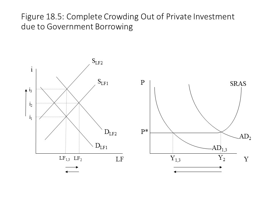 The reduction in the supply of loanable funds causes a leftward shift of the supply curve, which drives the interest rate up further but causes the equilibrium quantity exchanged to return to its original level. The refusal of the central bank to accommodate the increase in government borrowing has led to a higher interest rate, which completely crowds out debt-financed private investment and consumption. That is, government spending on goods and services expands entirely at the expense of private sector spending on goods and services. In terms of the AD/AS model, the increase in debt-financed government spending will increase aggregate demand, but the higher interest rates reduce investment spending and consumer spending, which leaves AD unchanged in the end as shown in Figure 18.5. In this scenario involving complete crowding out of private investment, the composition of total output changes with a shift away from investment spending and towards government spending, but the aggregate output is not affected.[4] It is also worth noting that the multiplier effect is completely inoperative in this situation even though the price level is constant.
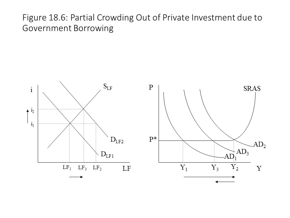 The increased demand for loanable funds in Figure 18.6 causes the interest rate and the quantity exchanged to increase. Although the interest rate rises, it does not rise as much as it does when the central bank also restricts the supply of loanable funds. This scenario involves the partial crowding out of private investment spending and private consumer spending because the higher demand does manage to increase the equilibrium quantity in this market even as the interest rate rises. The partial crowding out is reflected in the movement along the new demand curve as the interest rate rises. In this case, the increase in government spending shifts the AD curve to the right, which then partially shifts back to the left due to the reduction in consumer spending and investment spending as the interest rate rises. The multiplier effect is lessened in this situation as well due to the rise in interest rates even though the price level is constant.
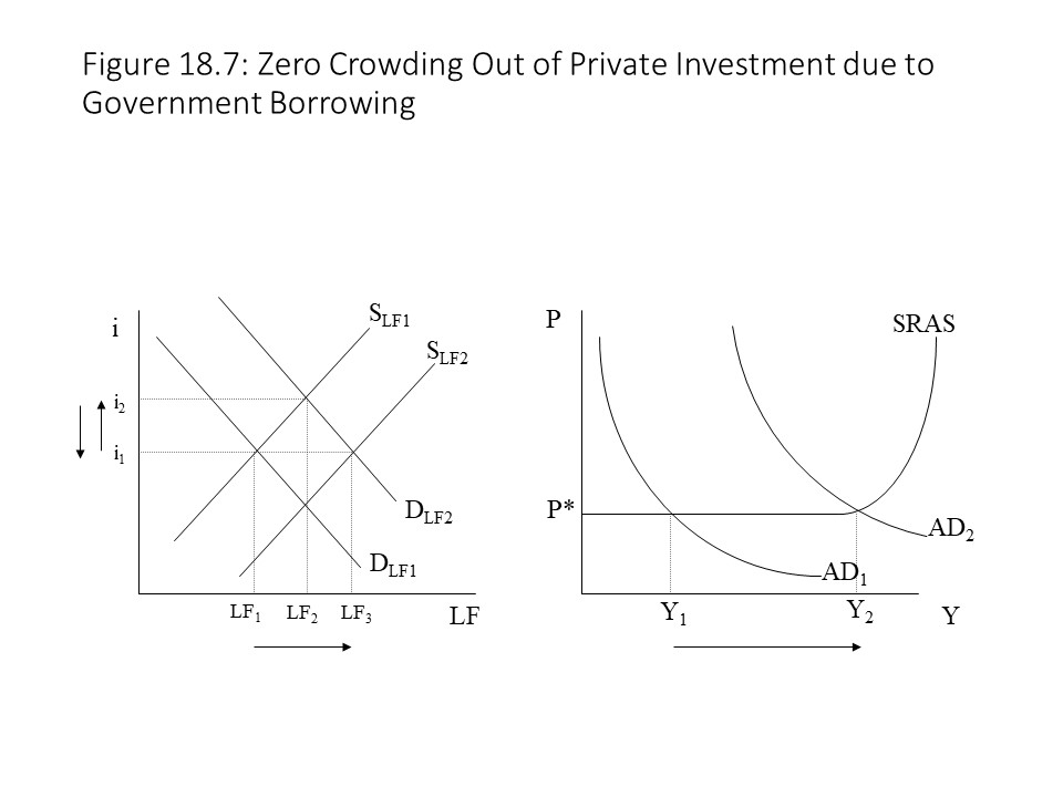 In Figure 18.7 the demand for loanable funds increases due to government borrowing, but then the supply of loanable funds also rises as the central bank accommodates the increased demand for loans. The rightward shift of the demand curve raises the equilibrium quantity and the interest rate. The rightward shift of the supply further raises the equilibrium quantity but brings the interest rate back down to the original level. Because the interest rate does not change in this situation, no crowding out of private investment or private consumption occurs, and the full multiplier effect is operative if the price level is constant. This scenario was discussed in Chapter 17 in the context of Post-Keynesian endogenous money supply theory. The Fed accommodates the higher demand for loanable funds with an increase in the money supply. If prices are sticky, then the full impact of the higher money supply is felt on real output. If the rightward shift of AD occurred in the upward sloping portion of the SRAS curve, then the rise in the price level would lessen the impact on real output. Even with a rise in the price level, however, no crowding out occurs because the interest rate does not rise.
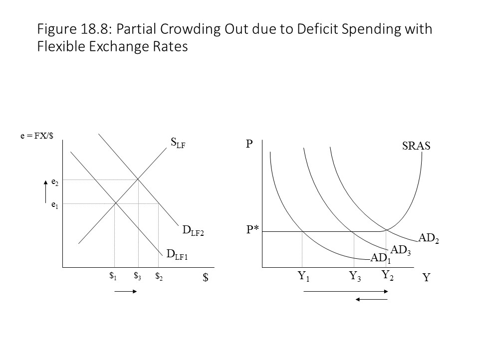 When the dollar appreciates, U.S. exports become more expensive for foreign buyers and imports become cheaper for American buyers. The consequence is a reduction in U.S. exports and a rise in U.S. imports. Net exports thus fall, which causes a leftward shift of the AD curve, partially offsetting the rightward shift of AD due to higher government spending.
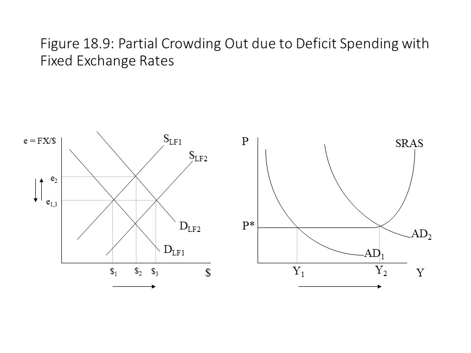 If the exchange rate returns to its original level, then net exports should not be negatively affected even though the government deficit spending will still lead to a rise in interest rates and partial crowding out. The partial crowding out in this case would involve a leftward shift of AD from AD2 (not shown in the graph), but the shift would not be as large as that shown in Figure 18.8 because a reduction in net exports does not contribute to the decline in aggregate demand in this case.
 The consequence of the central bank’s supply reduction is a further appreciation of the U.S. dollar even as it stabilizes the quantity exchanged of dollars. Figure 18.10 assumes that the crowding out of private investment and the negative impact on net exports exactly offset the expansionary impact of the deficit spending. The impact on U.S. net exports could be so extreme, however, that combined with the partial crowding out of private investment, the consequent drop in real output and employment could more than cancel the expansionary impact of the government deficit spending.
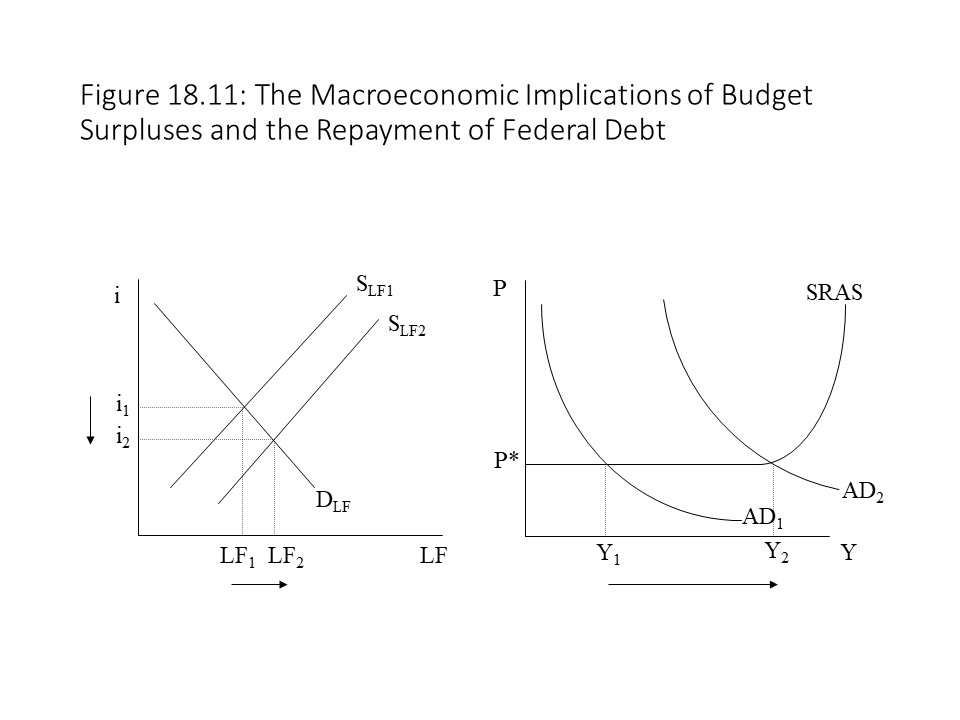
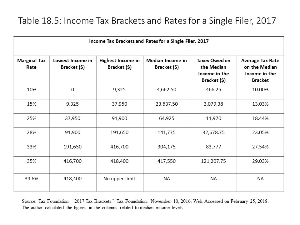
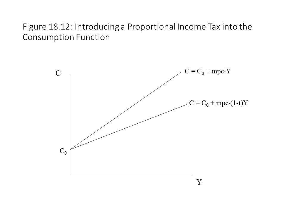 This result is very different from the situation involving a lump sum tax. In that situation, explored in Chapter 13, the imposition of the lump sum tax causes a downward parallel shift of the consumption line because the vertical intercept falls.
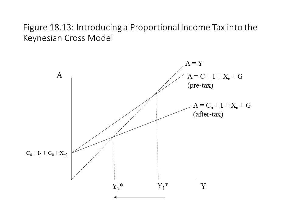 Figure 18.13 shows that the flatter A curve implies a lower equilibrium level of real output. The reader should recall that the equilibrium output level in the Keynesian Cross model occurs where planned aggregate spending is equal to real output (A=Y). This condition is met where the aggregate expenditures curve intersects the 45-degree line in the graph. A higher tax rate would cause aggregate spending to fall even further and would further reduce real output and employment. On the other hand, a lower flat tax rate would represent an expansionary fiscal policy. It would make the A curve steeper and would raise the equilibrium output and level of employment.
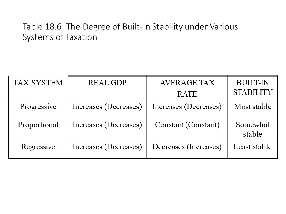 Table 18.6 shows how the average tax rate changes as real GDP (real income) changes under each of the three systems of taxation. It is asserted that progressive tax systems are the most stable taxation system and that proportional tax systems are somewhat stable. Regressive tax systems are regarded as the least stable system of taxation.
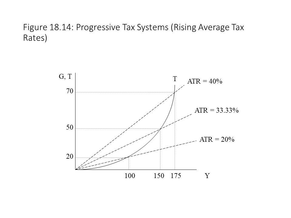 In Figure 18.14, tax revenues rise very quickly as real income rises, which causes the ratio of taxes paid to income to grow quickly. The steeply rising T line implies a rising marginal tax rate (MTR) and a rising average tax rate (ATR). Each of these tax rates may be defined as follows:
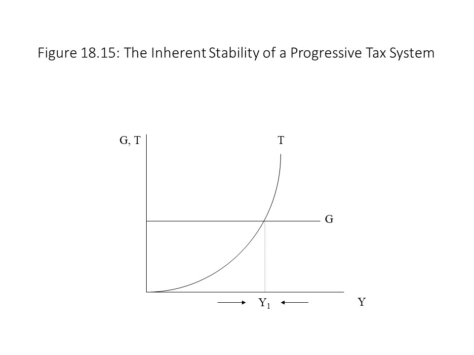 Figure 18.15 shows that the two curves intersect at Y1, which implies that the budget is balanced with G equal to T. At income levels below Y1, however, a government budget deficit exists. At income levels above Y1 a government budget surplus exists. Now suppose that the economy begins at income level, Y1, and a recession occurs. Because budget deficits have an expansionary impact on the economy due to high government spending relative to tax revenues, the economy has an automatic tendency to expand. Similarly, if the economy begins at Y1 and an expansion occurs, then the budget surplus that results has a contractionary impact on the economy due to low government spending relative to tax revenues.
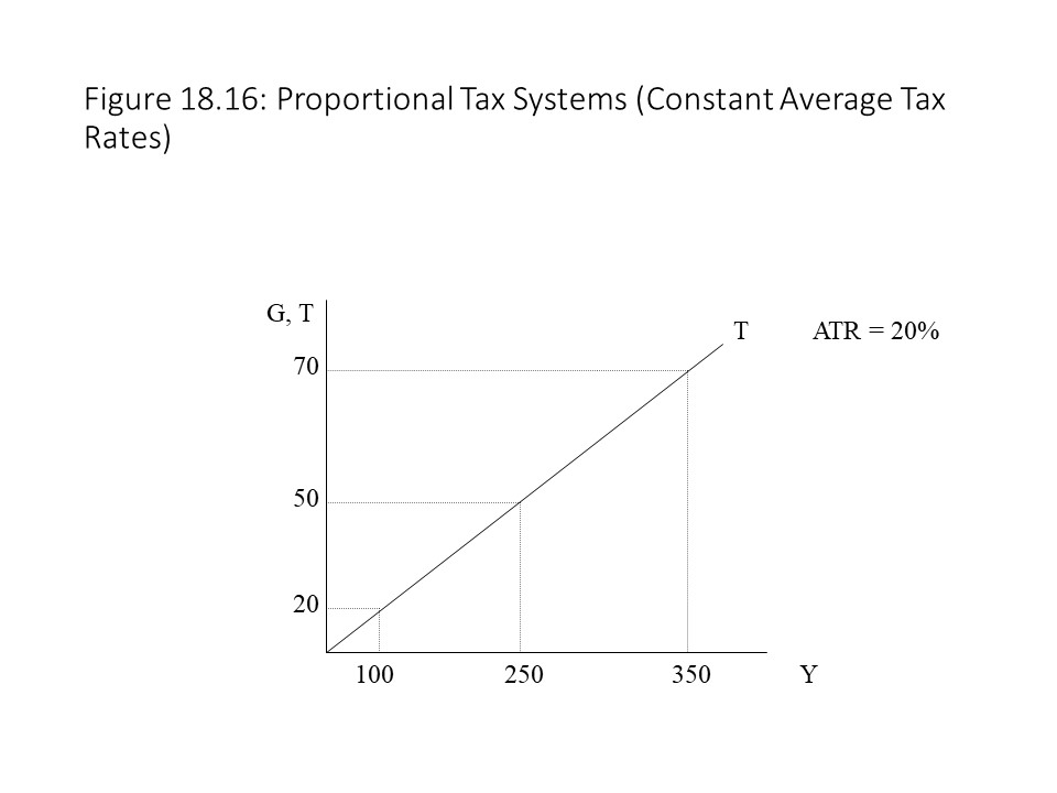 In Figure 18.16, tax revenues rise at a constant rate relative to income, which causes the ratio of taxes paid to income to remain stable. The linear T line implies a constant marginal tax rate (MTR) and a constant average tax rate (ATR).
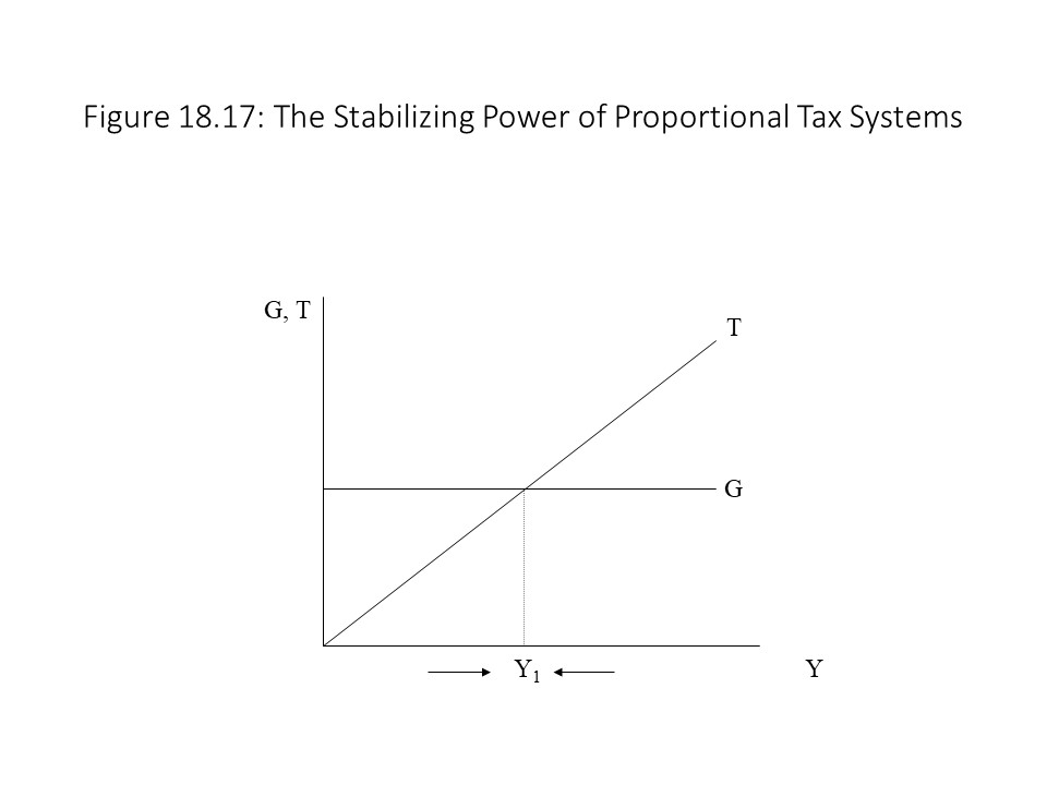 Figure 18.17 shows that the two curves intersect at Y1, which implies that the budget is balanced with G equal to T. At income levels below Y1, however, a government budget deficit exists. At income levels above Y1 a government budget surplus exists. Now suppose that the economy begins at income level, Y1, and a recession occurs. Because budget deficits have an expansionary impact on the economy due to high government spending relative to tax revenues, the economy has an automatic tendency to expand. Similarly, if the economy begins at Y1 and an expansion occurs, then the budget surplus that results has a contractionary impact on the economy due to low government spending relative to tax revenues.
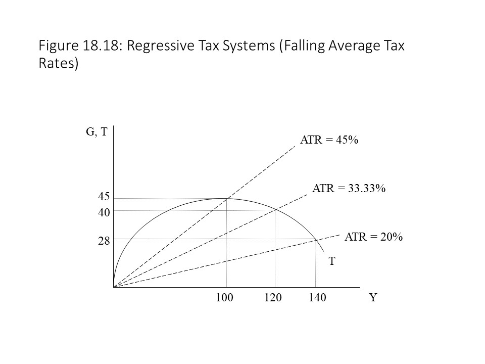 In Figure 18.18, tax revenues rise and then fall as real income increases, which causes the ratio of taxes paid to income to fall. The inverted-U shape of the T line implies a falling MTR and a falling ATR.
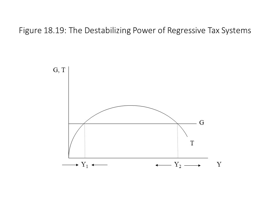 Figure 18.19 shows that the two curves intersect at two points, Y1 and Y2, which implies that the budget is balanced at both income levels with G equal to T. At income levels below Y1, a budget deficit exists. At income levels above Y1 a government budget surplus exists. These results are identical to what we have observed in the case of a progressive tax system and a proportional tax system. If the economy moves away from Y1, then it has an automatic tendency to move back towards it.
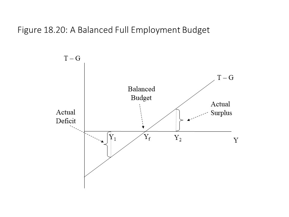
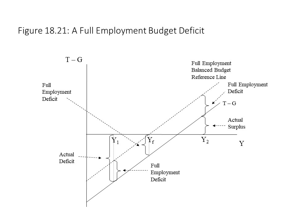
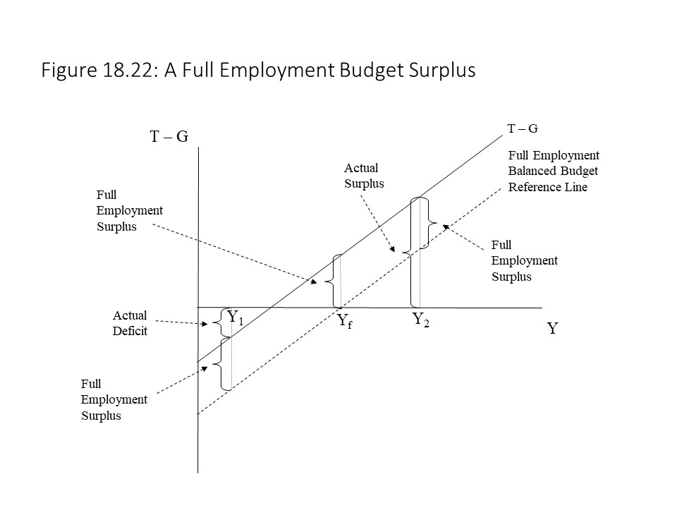
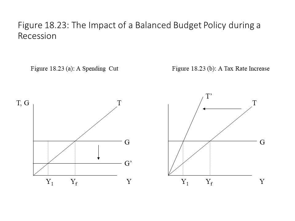 Figure 18.23 shows two methods of balancing the budget when output falls to Y1 and a budget deficit arises. In Figure 18.23 (a), a government spending cut will restore balance to the budget since tax revenues have fallen. The problem with this approach is that a government spending cut is a contractionary fiscal policy, which is likely to worsen the recession. A balanced budget is thus achieved but at great cost to the nation’s well-being. An alternative policy is to increase the average tax rate as shown in Figure 18.23 (b). In Figure 18.23 (b), tax revenues increase to restore balance to the budget, but a tax increase is also a contractionary policy taken during a recession. It seems that a balanced budget policy is likely to be a difficult and painful policy to pursue in a recession.
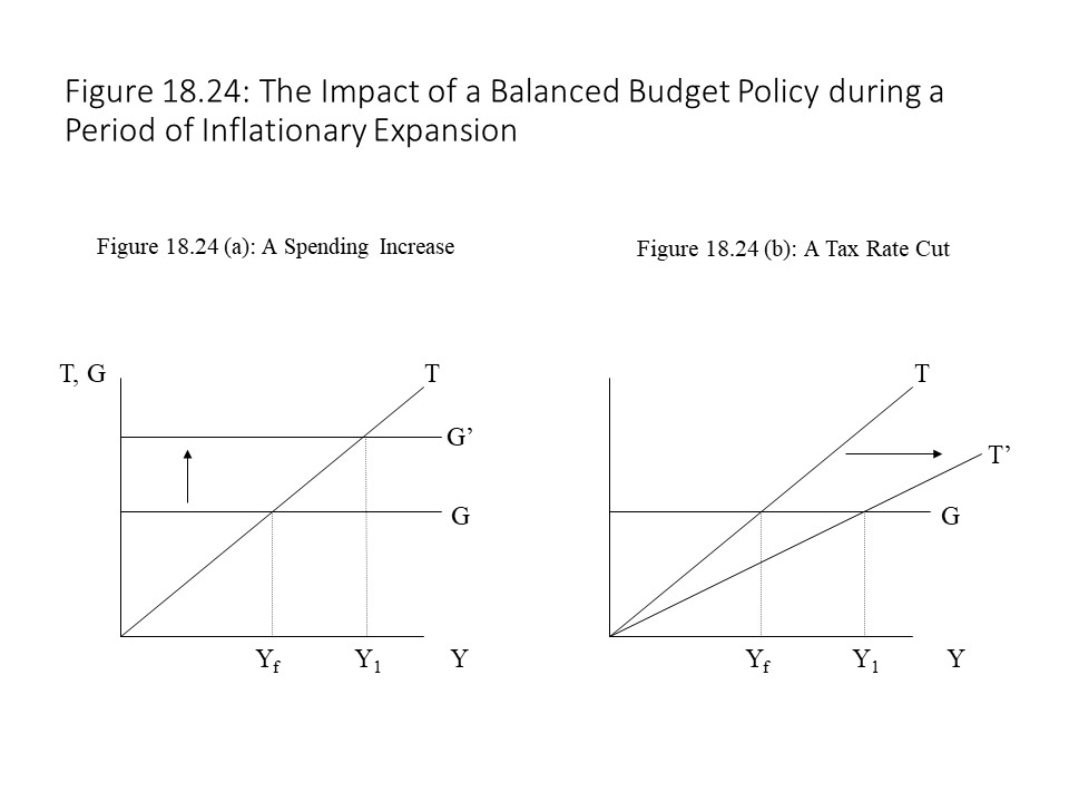
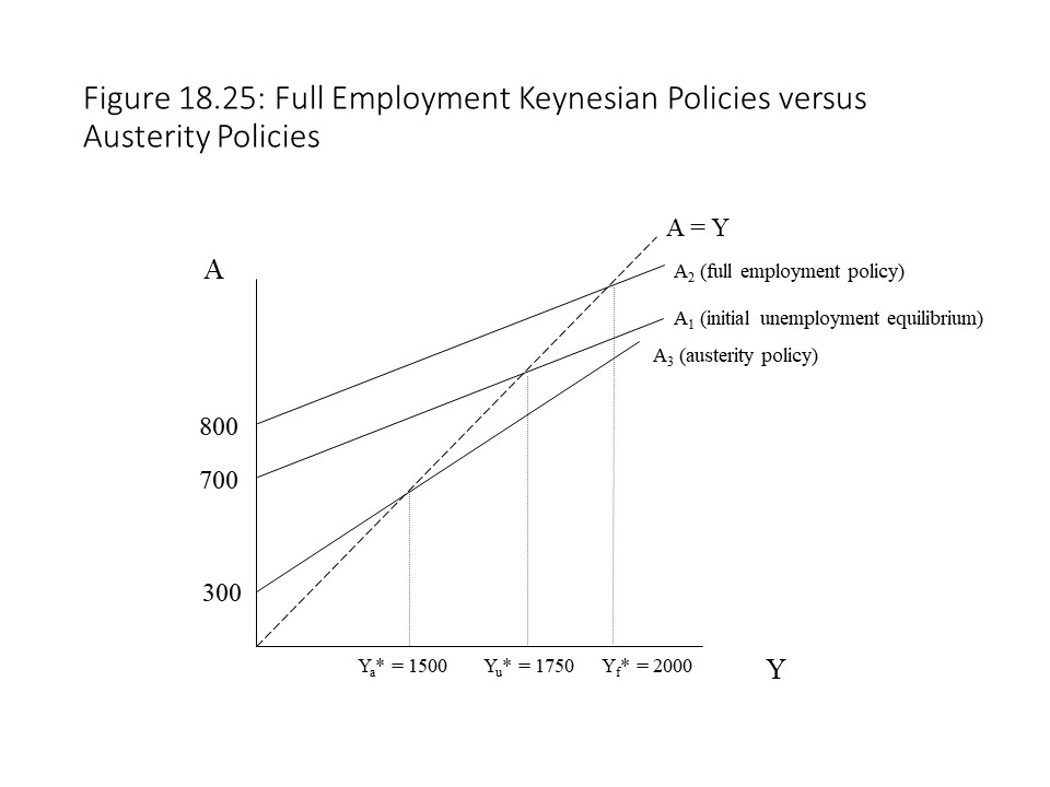
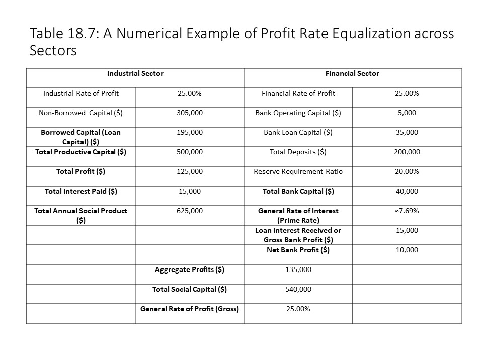 In the example shown in Table 18.7, the market rate of interest has adjusted to equal the general rate of interest. The adjustment of the interest rate is what makes possible the equalization of the rate of profit in this example. Using this case as a starting point, we will consider two scenarios involving government borrowing and the consequences that it carries for the economy.
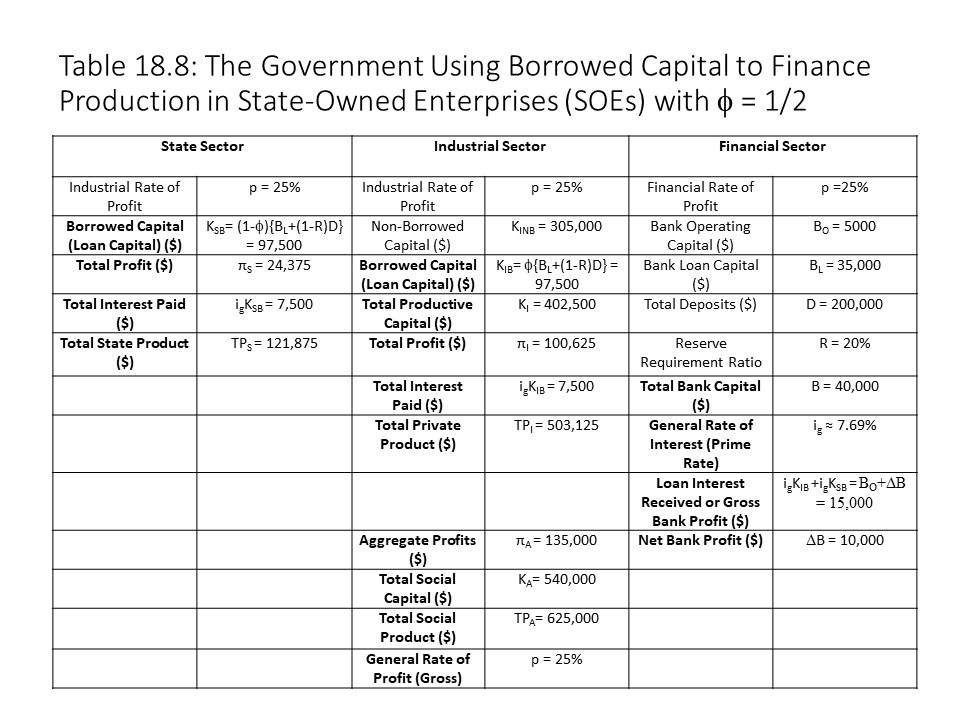
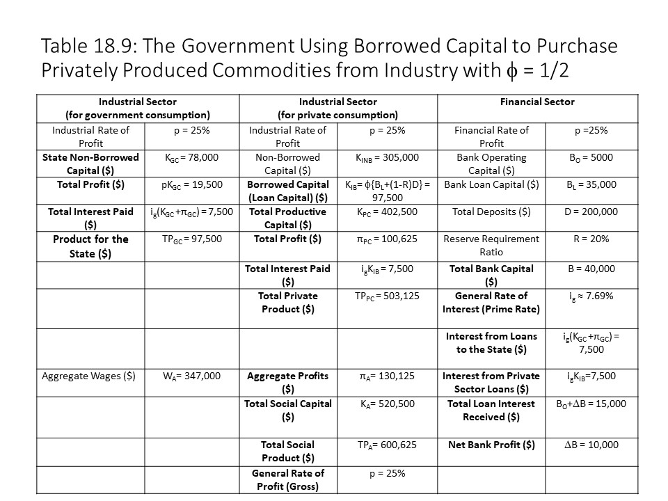
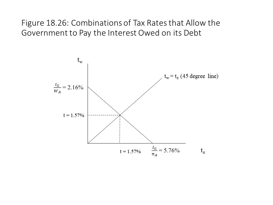 As Figure 18.26 shows, if only wages are taxed, then the tax rate on wages may be calculated simply by dividing the interest owed by the aggregate wage income. If only profits are taxed, then the tax rate on profits may be calculated simply by dividing the interest owed by the aggregate profit income. If both wages and profits are taxed at the same rate (t), then the tax rate is calculated by dividing the interest owed by the sum of all wages and profits. Finally, the slope indicates that a one percent increase in the tax rate on profits will cause a reduction in the tax rate on wages of πA/WA.