6.5: Inferential statistics for cardinal data

Where one variable is nominal (more precisely, nominal with two values) and one is cardinal, the a widely-used test is the t -test, of which there are two well known versions, Welch’s t -test and Student’s t -test, that differ in terms of the requirements that the data must meet in order for them to be applicable. In the following, I will introduce Welch’s t -test, which can be applied more broadly, although it still has some requirements that I will return to below.

6.5.1 Welch’s t -test

Let us return to the case study of the length of modifiers in the two English possessive constructions. Here is the research hypothesis again, paraphrased slightly from (15) and (16) in Chapter 5:

(12) H1 : The S -POSSESSIVE will be used with short modifiers, the OF -POSSESSIVE will be used with long modifiers.

Prediction: The mean LENGTH (in “number of words”) of modifiers of the S -POSSESSIVE should be smaller than that of the modifiers of the OF -POSSESSIVE.

The corresponding null hypothesis is stated in (13):

(13) H0 : There is no relationship between LENGTH and TYPE OF POSSESSIVE.

Prediction: There will be no difference between the mean length of the modifiers of the S -POSSESSIVE and the OF -POSSESSIVE.

Table 6.12 shows the length in number of words for the modifiers of the s - and of -possessives (as already reported in Table 5.9), together with a number of additional pieces of information that we will turn to next.

First, note that one case that was still included in Table 5.9 is missing: Example (b 19) from that Table, which had a modifier of length 20. This is treated here as a so-called outlier, i.e., a value that is so far away from the mean that it can be considered an exception. There are different opinions on if and when outliers should be removed that we will not discuss here, but for expository reasons alone it is reasonable here to remove it (and for our results, it would not have made a difference if we had kept it).

In order to calculate Welch’s t -test, we determine three values on the basis of our measurements of LENGTH: the number of measurements N, the mean length for each group (x̄), and a value called “sample variance” (s ² ). The number of measurements is easy to determine – we just count the cases in each group: 20 s -possessives and 24 of -possessives. We already calculated the mean lengths in Chapter 5: for the s -possessive, the mean length is 1.9 words, for the of -possessive it is 3.83 words. As we already discussed in Chapter 5, this difference conforms to our hypothesis: s -possessives are, on average, shorter than of -possessives.

The question is, again, how likely it is that this difference is due to chance. When comparing group means, the crucial question we must ask in order to determine this is how large the variation is within each group of measurements: put simply, the more widely the measurements within each group vary, the more likely it is that the differences across groups have come about by chance.

Table 6.12: Length of the modifier in the sample of s - and of -possessives from Table 5.9

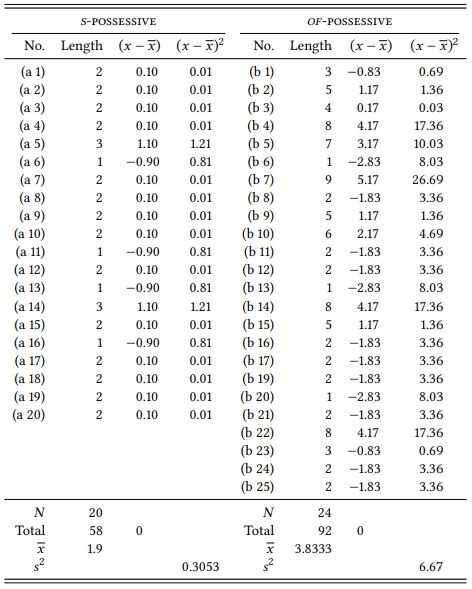
The first step in assessing the variation consists in determining for each measurement, how far away it is from its group mean. Thus, we simply subtract each measurement for the S -POSSESSIVE from the group mean of 1.9, and each measurement for the OF -POSSESSIVE from the group mean of 3.83. The results are shown in the third column of each sub-table in Table 6.12. However, we do not want to know how much each single measurement deviates from the mean, but how far the group S -POSSESSIVE or OF -POSSESSIVE as a whole varies around the mean. Obviously, adding up all individual values is not going to be helpful: as in the case of observed and expected frequencies of nominal data, the result would always be zero. So we use the same trick we used there, and calculate the square of each value – making them all positive and weighting larger deviations more heavily. The results of this are shown in the fourth column of each sub-table. We then calculate the mean of these values for each group, but instead of adding up all values and dividing them by the number of cases, we add them up and divide them by the total number of cases minus one. This is referred to as the sample variance:

(14)

The sample variances themselves cannot be very easily interpreted (see further below), but we can use them to calculate our test statistic, the t-value, using the following formula (x̄ stands for the group mean,s ² stands for the sample variance, and N stands for the number of cases; the subscripts 1 and 2 indicate the two subsamples:

(15)

Note that this formula assumes that the measures with the subscript 1 are from the larger of the two samples (if we don’t pay attention to this, however, all that happens is that we get a negative t -value, whose negative sign we can simply ignore). In our case, the sample of of -possessives is the larger one, giving us:

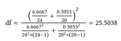
As should be familiar by now, we compare this t-value against its distribution to determine the probability of error (i.e., we look it up in the table in Section 14.4 in the Statistical Tables at the end of this book. Before we can do so, however, we need to determine the degrees of freedom of our sample. This is done using the following formula:

(16)

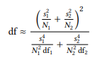
Again, the subscripts indicate the sub-samples, s ² is the sample variance, and N is the number of items the degrees of freedom for the two groups (df₁ and df₂ ) are defined as N − 1. If we apply the formula to our data, we get the following:

As we can see in the table of critical values, the t -value is smaller than 0.01. A t -test should be reported in the following format:

(17) Format for reporting the results of a t test

(t([deg. freedom]) = [t value], p < (or >) [sig. level]).

Thus, a straightforward way of reporting our results would be something like this: “This study has shown that for modifiers that are realized by lexical NPs, s -possessives are preferred when the modifier is short, while of -possessives are preferred when the modifier is long. The difference between the constructions is very significant (t(25.50) = 3.5714, p < 0.01)”.

As pointed out above, the value for the sample variance does not, in itself, tell us very much. We can convert it into something called the sample standard deviation, however, by taking its square root. The standard deviation is an indicator of the amount of variation in a sample (or sub-sample) that is frequently reported; it is good practice to report standard deviations whenever we report means.

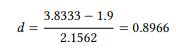
Finally, note that, again, the significance level does not tell us anything about the size of the effect, so we should calculate an effect size separately. The most widely-used effect size for data analyzed with a t -test is Cohen’s d, also referred to as the standardized mean difference. There are several ways to calculate it, the simplest one is the following, where σ is the standard deviation of the entire sample:

(18)

For our case study, this gives us

This standardized mean difference can be converted to a correlation coefficient by the formula in (19):

(19)

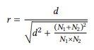
For our case study, this gives us

Since this is a correlation coefficient, it can be interpreted as described in Table 6.6 above. It falls into the moderate range, so a more comprehensive way of summarizing the results of this case study would be the following: “This study has shown that length has a moderate, statistically significant influence on the choice of possessive constructions with lexical NPs in modifier position: s -possessives are preferred when the modifier is short, while of -possessives are preferred when the modifier is long. (t(25.50) = 3.5714, p < 0.01, r = 0.41)”.

6.5.2 Normal distribution requirement

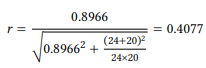
In the context of corpus linguistics, there is one fundamental problem with the t -test in any of its variants: it requires data that follow what is called the normal distribution. Briefly, the normal distribution is a probability distribution where most measurements fall in the middle, decreasing on either side until they reach zero. Figure 6.1a shows some examples. As you can see, the curve may be narrower or wider (depending on the standard deviation) and it may be positioned at different points on the x axis (depending on the mean), but it is always a symmetrical bell curve.

You will often read that many natural phenomena approximate this distribution – examples mentioned in textbooks are, invariably, the size and weight of organisms, frequently other characteristics of organisms such as skin area, blood pressure or IQ, and occasionally social phenomena like test scores and salaries. Figure 6.1b show the distribution of body weight in a sample of swans collected for an environmental impact study (Fite 1979), and, indeed, it seems to follow, roughly, a normal distribution if we compare it to the bell curve superimposed on the figure.

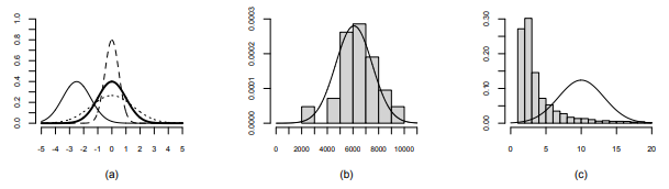
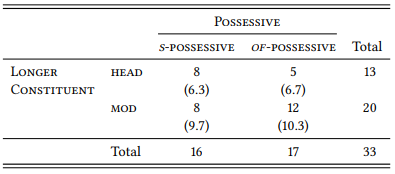
Figure 6.1: The normal distribution and linguistic data

Unfortunately, cardinal measurements derived from language data (such as the length or of words, constituents, sentences, etc. or the distance to the last mention of a referent) are rarely (if ever) normally distributed (see, e.g., McEnery & Hardie 2012: 51). Figure 6.1c shows the distribution of the constituent length, in number of words, of of -phrases modifying nouns in the SUSANNE corpus (with of -phrases with a length of more than 20 words removed as outliers). As you can see, they do not follow a normal distribution at all – there are many more short of -phrases than long ones, shifting the distribution further to the left and making it much narrower than it should be.

There are three broad ways of dealing with this issue. First, we could ignore it and hope that the t -test is robust enough to yield meaningful results despite this violation of the normality requirement. If this seems like a bad idea, this is because it is fundamentally a bad idea – and statisticians warn against it categorically. However, many social scientists regularly adopt this approach – just like we did in the case study above. And in practice, this may be less of a problem than one might assume, since the t -test has been found to be fairly robust against violations of the normality requirement. However, we should not generally rely on this robustness, as linguistic data may depart from normality to quite an extreme degree. More generally, ignoring the prerequisites of a statistical procedure is not exactly good scientific practice – the only reason I did it above was so you would not be too shocked when you see it done in actual research (which, inevitably, you will).

Second, and more recommendably, we could try to make the data fit the normality requirement. One way in which this is sometimes achieved in the many cases where data do not follow the normal distribution is to log-transform the data (i.e., use the natural logarithm of the data instead of the data themselves). This often, but not always, causes the data to approximate a normal distribution more closely. However, this does not work in all cases (it would not, for example, bring the distribution in Figure 6.1c much closer to a normal distribution, and anyway, transforming data carries its own set of problems.

Thus, third, and most recommendably, we could try to find a way around having to use a t -test in the first place. One way of avoiding a t -test is to treat our non-normally distributed cardinal data as ordinal data, as described in Chapter 5. We can then use the Mann-Whitney U -test, which does not require a normal distribution of the data. I leave it as an exercise to the reader to apply this test to the data in Table 6.12 (you know you have succeeded if your result for U is 137, p < 0.01).

Another way of avoiding the t -test is to find an operationalization of the phenomenon under investigation that yields rank data, or, even better, nominal data in the first place. We could, for example, code the data in Table 6.12 in terms of a very simple nominal variable: LONGER CONSTITUENT (with the variables HEAD and MODIFIER). For each case, we simply determine whether the head is longer than the modifier (in which case we assign the value head) or whether the modifier is longer than the head (in which case we assign the value MODIFIER; we discard all cases where the two have the same length. This gives us Table 6.13.

Table 6.13: The influence of length on the choice between the two possessives

The χ² value for this table is 0.7281, which at one degree of freedom means that the p value is larger than 0.05, so we would have to conclude that there is no influence of length on the choice of possessive construction. However, the deviations of the observed from the expected frequencies go in the right direction, so this may simply be due to the fact that our sample is too small (obviously, a serious corpus-linguistic study would not be based on just 33 cases).

The normal-distribution requirement is only one of several requirements that our data set must meet in order for particular statistical methods to be applicable.

For example, many procedures for comparing group means – including the more widely-used Student t -test – can only be applied if the two groups have the same variance (roughly, if the measurements in both groups are spread out from the group means to the same extent), and there are tests to tell us this (for example, the F test). Also, it makes a difference whether the two groups that we are comparing are independent of each other (as in the case studies presented here), or if they are dependent in that there is a correspondence between measures in the two groups. For example, if we wanted to compare the length of heads and modifiers in the s-possessive, we would have two groups that are dependent in that for any data point in one of the groups there is a corresponding data point in the other group that comes from the same corpus example. In this case, we would use a paired test (for example, the matched-pairs Wilcoxon test for ordinal data and Student’s paired t -test for cardinal data).