10.1: Introduction

From the early 1900s, ecologists have understood the population of a species as typically developing according to the S-curve shown in Figure 10.1. Consider a population that, with abundant resources, can double in one reproduction cycle. Two individuals become four over the first cycle. Those four become eight over the second cycle. Note that in the first cycle only two individuals were added, while four were added in the same amount of time in the second cycle. As the doubling continues, the population will reach 16, 32, 64, 128 and so on. This rapid increase explains the first half of the S-curve in Figure 10.1, as it moves from very shallow to very steep increases. This rapid increase in population is called exponential growth.

Figure 10.1: Carrying capacity. S-curve model for growth of population.

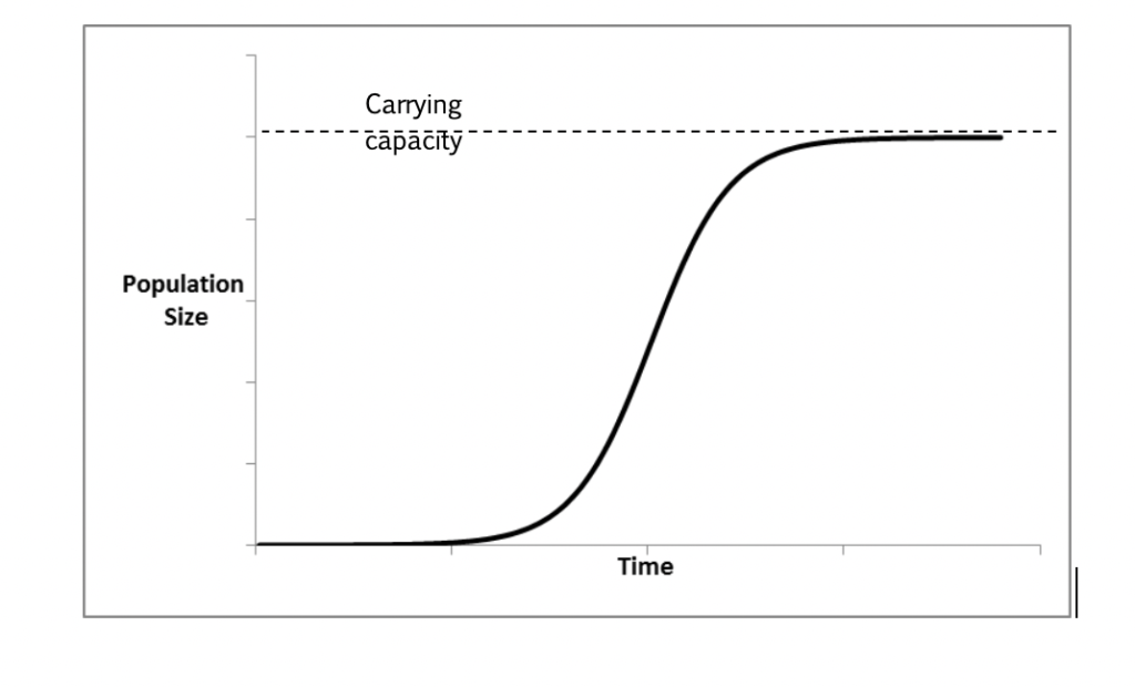
According to this model, the population will continue to grow exponentially until it reaches the limits dictated by available resources (food, space, etc.). As the amount of available resources per individual declines—in other words, as resources become scarce—mortality rates increase and reproductive rates decrease, causing the population to level off at what ecologists call the “carrying capacity” of an ecosystem—the maximum population size that an ecosystem can support sustainably. Many have applied this same basic model to humans as well, pointing toward localized examples of resource scarcity as evidence that humans are subject to the same ecological realities observed in other species. This claim has proven controversial in part because of people’s general aversion to being lumped in with other species. Some argue that our ingenuity and adaptability as a species allows us to transcend ecological barriers that constrain other species. Indeed, human population dynamics have shown that the carrying capacity of an ecosystem (or of the global system) may not be as fixed as ecologists once assumed. We will return to this topic later, but first, let’s take a look at how earlier societies have addressed resource challenges.

Incidentally, the same S-shaped curve (or part of it, as of yet) is observed in plots of resource use over time, economic production, energy use, fertiliser consumption, transportation, communication, tourism, pollution, deforestation and other forms of land degradation. Those plots gave rise to the concept of the Great Acceleration (Steffen et al., 2015) that introduced the Anthropocene. The point is that while the population is growing exponentially, many of its activities do so as well. This even goes for plots per capita, at least temporarily! Sooner or later, however, limiting factors become operative, slowing the increase until an inflection point is passed and further slowing results in a plateau – or even a crash. Quite often those ‘limiting factors’ amount to resource scarcity.