This chapter has introduced you to the forces of evolution, the mechanisms by which evolution occurs. How do we detect and study evolution, though, in real time, as it happens? One tool we use is the : a mathematical formula that allows estimation of the number and distribution of dominant and recessive alleles in a population. This aids in determining whether allele frequencies are changing and, if so, how quickly over time, and in favor of which allele? It’s important to note that the Hardy-Weinberg formula only gives us an estimate based on the data for a snapshot in time. We will have to calculate it again later, after various intervals, to determine if our population is evolving and in what way the allele frequencies are changing. To learn how to calculate the Hardy-Weinberg formula, see the Special Topic box at the end of the chapter.
Interpreting Evolutionary Change
Once we have detected change occurring in a population, we need to consider which evolutionary processes might be the cause of the change. It is important to watch for non-random mating patterns, to see if they can be included or excluded as possible sources of variation in allele frequencies.
Non-Random Mating
(also known as Assortative Mating) occurs when mate choice within a population follows a non-random pattern. Positive assortative mating patterns result from a tendency for individuals to mate with others who share similar phenotypes. This often happens based on body size. Taking as an example dog breeds, it is easier for two Chihuahuas to mate and have healthy offspring than it is for a Chihuahua and a St. Bernard to do so. This is especially true if the Chihuahua is the female and would have to give birth to giant St. Bernard pups.
Negative assortative mating patterns occur when individuals tend to select mates with qualities different from their own. This is what is at work when humans choose partners whose pheromones indicate that they have different and complementary immune alleles, providing potential offspring with a better chance at a stronger immune system.
Among domestic animals, such as pets and livestock, assortative mating is often directed by humans who decide which pairs will mate to increase the chances of offspring having certain desirable traits. This is known as artificial selection.
Among humans, in addition to phenotypic traits, cultural traits such as religion and ethnicity may also influence assortative mating patterns.
Micro- to Macroevolution
Microevolution refers to changes in allele frequencies within breeding populations, that is, within single species. Macroevolution involves changes that result in the emergence of new species, the similarities and differences between species and their phylogenetic relationships with other taxa. Consider our example of the peppered moth which illustrated microevolution over time, via directional selection favoring the peppered allele when the trees were clean and the dark pigment allele when the trees were sooty. Imagine that environmental regulations had cleaned up the air pollution in one part of the nation, while the coal-fired factories continued to spew soot in another area. If this went on long enough, it’s possible that two distinct moth populations would eventually emerge—one containing only the peppered allele and the other only harboring the dark pigment allele.
When a single population divides into two or more separate species, it is called speciation. The changes that prevent successful breeding between individuals who descended from the same ancestral population may involve chromosomal rearrangements, changes in the ability of the sperm from one species to permeate the egg membrane of the other species, or dramatic changes in hormonal schedules or mating behaviors that prevent members from the new species from being able to effectively pair up.
There are two types of speciation: allopatric and sympatric. Allopatric speciation is caused by long-term isolation (physical separation) of subgroups of the population (Figure 4.19). Something occurs in the environment—perhaps a river changes its course and splits the group, preventing them from breeding with members on the opposite riverbank. Over many generations, new mutations and adaptations to the different environments on each side of the river may drive the two subpopulations to change so much that they can no longer produce fertile, viable offspring, even if the barrier is someday removed.
Figure \(\PageIndex{1}\): Isolation leading to speciation: (a) original population before isolation; (b) a barrier divides the population and prevents interbreeding between the two groups; (c) time passes, and the populations become genetically distinct; (d) after many generations, the two populations are no longer biologically or behaviorally compatible, thus can no longer interbreed, even if the barrier is removed.
Sympatric speciation occurs when the population splits into two or more separate species while remaining located together without a physical barrier. This typically results from a new mutation that pops up among some members of the population that prevents them from successfully reproducing with anyone who does not carry the same mutation. This is seen particularly often in plants, as they have a higher frequency of chromosomal duplications.
One of the quickest rates of speciation is observed in the case of adaptive radiation. Adaptive radiation refers to the situation in which subgroups of a single species rapidly diversify and adapt to fill a variety of ecological niches. An ecological niche is a set of constraints and resources that is available in an environmental setting. Evidence for adaptive radiations is often seen after population bottlenecks. A mass disaster kills off many species, and the survivors have access to a new set of territories and resources that were either unavailable or much coveted and fought over before the disaster. The offspring of the surviving population will often split into multiple species, each of which stems from members in that first group of survivors who happened to carry alleles that were advantageous for a particular niche.
The classic example of adaptive radiation brings us back to Charles Darwin and his observations of the many species of finches on the Galapagos Islands. We are still not sure how the ancestral population of finches first arrived on that remote Pacific Island chain, but they found themselves in an environment filled with various insects, large and tiny seeds, fruit, and delicious varieties of cactus. Some members of that initial population carried alleles that gave them advantages for each of these dietary niches. In subsequent generations, others developed new mutations, some of which were beneficial. These traits were selected for, making the advantageous alleles more common among their offspring. As the finches spread from one island to the next, they would be far more likely to find mates among the birds on their new island. Birds feeding in the same area were then more likely to mate together than birds who have different diets, contributing to additional assortative mating. Together, these evolutionary mechanisms caused rapid speciation that allowed the new species to make the most of the various dietary niches (Figure 4.20).
In today’s modern world, understanding these evolutionary processes is crucial for developing immunizations and antibiotics that can keep up with the rapid mutation rate of viruses and bacteria. This is also relevant to our food supply, which relies, in large part, on the development of herbicides and pesticides that keep up with the mutation rates of pests and weeds. Viruses, bacteria, agricultural pests, and weeds have all shown great flexibility in developing alleles that make them resistant to the latest medical treatment, pesticide, or herbicide. Billion-dollar industries have specialized in trying to keep our species one step ahead of the next mutation in the pests and infectious diseases that put our survival at risk.
SPECIAL TOPIC: CALCULATING THE HARDY-WEINBERG EQUILIBRIUM
In the Hardy-Weinberg formula, p represents the frequency of the dominant allele, and q represents the frequency of the recessive allele. Remember, an allele’s frequency is the proportion, or percentage, of that allele in the population. For the purposes of Hardy-Weinberg, we give the allele percentages as decimal numbers (e.g., 42% = 0.42), with the entire population (100% of alleles) equaling 1. If we can figure out the frequency of one of the alleles in the population, then it is simple to calculate the other. Simply subtract the known frequency from 1 (the entire population). Therefore: 1 – p = q and 1 – q = p
The Hardy-Weinberg formula is p2 + 2pq + q2, where
p2 represents the frequency of the homozygous dominant genotype;
2pq represents the frequency of the heterozygous genotype; and
q2 represents the frequency of the homozygous recessive genotype.
It is often easiest to determine q2 first, simply by counting the number of individuals with the unique, homozygous recessive phenotype (then dividing by the total individuals in the population to arrive at the “frequency”). If we can do this, we simply need to calculate the square root of the homozygous recessive phenotype frequency. That gives us q. Remember, 1 –q equals p, so now we have the frequencies for both alleles in the population. If we needed to figure out the frequencies of heterozygotes and homozygous dominant genotypes, we’d just need to plug the p and q frequencies back into the p2 and 2pq formulas.
Figure \(\PageIndex{3}\): Ladybug population with a mixture of dark (red) and light (orange) individuals.
Let’s imagine we have a population of ladybeetles that carries two alleles: a dominant allele that produces red ladybeetles and a recessive allele that produces orange ladybeetles. Since red is dominant, we’ll use R to represent the red allele, and r to represent the orange allele. Our population has ten beetles, and seven are red and three are orange (Figure 4.21). Let’s calculate the number of genotypes and alleles in this population.
We have three orange beetles of our ten, 3/10 = .30 (30%) frequency, and we know they are homozygous recessive (rr). So:
rr = .3; therefore, r = √.3 = .5477
R = 1 – .5477 = .4523
Using the Hardy-Weinberg formula:
1=.45232 + 2 x .4523 x .5477 +.54772 = .20 + .50 + .30 = 1
Thus, the genotype breakdown is 20% RR, 50% Rr, and 30% rr
(2 red homozygotes, 5 red heterozygotes, and 3 orange homozygotes).
Since we have 10 individuals, we know we have 20 total alleles: 4 red from the RR group, 5 red and 5 orange from the Rr group, and 6 orange from the rr group, for a grand total of 9 red and 11 orange (45% red and 55% orange, just like we estimated in the 1 – q step).
Reminder: The Hardy-Weinberg formula only gives us an estimate for a snapshot in time. We will have to calculate it again later, after various intervals, to determine if our population is evolving and in what way the allele frequencies are changing.
Review Questions
You inherit a house from a long-lost relative that contains a fancy aquarium, filled with a variety of snails. The phenotypes include large snails and small snails; red, black, and yellow snails; and solid, striped, and spotted snails. Devise a series of experiments that would help you determine how many snail species are present in your aquarium.
The many breeds of the single species of domestic dog (Canisfamiliaris) provide an extreme example of microevolution. Discuss why this is the case. What future scenarios can you imagine that could potentially transform the domestic dog into an example of macroevolution?
The ability to roll one’s tongue (lift the outer edges of the tongue to touch each other, forming a tube) is a dominant trait. In small town of 1,500 people, 500 can roll their tongues. Use the Hardy-Weinberg formula to determine how many individuals in the town are homozygous dominant, heterozygous, and homozygous recessive.
Match the correct force of evolution with the correct real-world example:

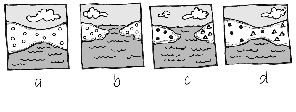
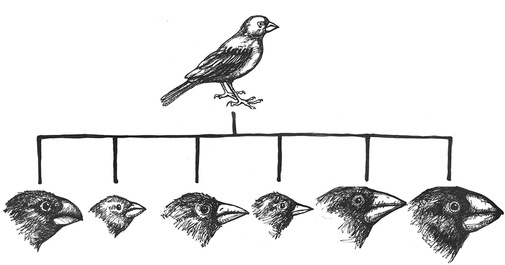
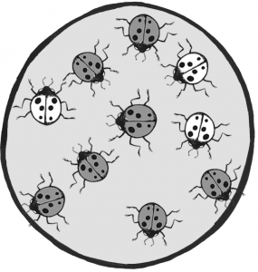 Figure \(\PageIndex{3}\): Ladybug population with a mixture of dark (red) and light (orange) individuals.