9.6: Consumption Function

Of the four sources of demand (C, I, G, and NX), consumption demand (C) is the largest in developed economies. In the United States, consumption demand (sometime referred to as household consumption) represents about 68% of all demand. So, if policy makers want to move the economy to full employment by shifting the AD curve, it makes sense to stimulate the largest demand component. 

Household demand is driven by income. When income increases the demand for most goods also increases. The converse is also true. When income decreases the demand for most goods decreases. 

John Keynes recognized that if the goal is to stimulate aggregate demand, the most effective strategy is to increase household income. He understood that when people have more income, they are more likely to spend on goods and services, creating a ripple effect throughout the economy. By focusing on boosting employment and wages - through government spending or targeted fiscal policies (fiscal policy will be discuss in later chapters) - Keynes believed policymakers could raise incomes, fuel demand, and pull the economy out of recession. 

Figure 11 

Figure 11 shows the change in real personal consumption expenditures (i.e., household spending on new goods and services) and disposable income from 2010 to 2024. Clearly, household consumption rises with income. 

Consumption and Savings in Relation to Income

Disposable income is the foundation of both consumption (spending) and saving decisions. Disposable income is the amount of income that households have left to spend or save after paying taxes. From this point on disposable income and income will be used interchangeably. When individuals and families receive income, they make choices about how much to spend on goods and services and how much to save for future needs. As income increases, consumption also increases, but not by the full amount of income gain. This is because people tend to save a portion of any additional income. 

\[Y_D=C+S \nonumber\]

\(Y_D\) = Disposable Income  

\(C\) = Consumption  

\(S\) = Savings 

Marginal Propensity to Consume (MPC)

This relationship is captured by a concept called the Marginal Propensity to Consume (MPC). The MPC measures the fraction of each additional dollar of income that is spent on consumption. For example, if a household receives an extra $1 and spends $0.75 of it, the MPC is 0.75. The remaining $0.25 is saved, which corresponds to a Marginal Propensity to Save (MPS) of 0.25. See figure 12 

Figure 12 

We can use the following formula to calculate MPC: 

\[M P C=\frac{\Delta \mathrm{C}}{\Delta Y_D} \nonumber \]

\(\Delta \mathrm{C}\) = change in consumption 

\(\Delta Y_D\) = change in disposable income 

Understanding the MPC is essential when analyzing macroeconomic policy, especially policies designed to stimulate the economy. If the government increases spending or cuts taxes to boost household income, the effect on aggregate demand (AD) depends on how much of that new income is spent. The higher the MPC, the greater the impact on AD, because more of the stimulus flows through the economy as increased consumption. This is the basis for calculating the fiscal multiplier, which shows how an initial change in spending leads to a larger overall change in output and income. 

Consumption Function

We have already established that there is a relationship between consumption and income: as people’s incomes rise, they tend to spend more. This is a fundamental concept in macroeconomics, and it reflects the idea that consumption is positively related to disposable income. However, income is not the only factor that influences consumption. Even when income is zero, people still need to buy necessities - food, shelter, utilities, and other basic goods. This leads us to an important idea in macroeconomic theory: autonomous consumption. 

Autonomous consumption refers to the level of consumption that occurs even when income is zero. It is called “autonomous” because it does not depend on the current level of income. Instead, it may be influenced by factors such as borrowing, savings, expectations about the future, or government assistance. For example, a household may still spend money on rent and groceries by using savings or credit cards, even if no one in the household currently has a job. 

We use this concept to construct the consumption function, which is a mathematical model that describes total consumption as the sum of two parts: 

1. Autonomous consumption – the part of spending that happens regardless of income 
2. Induced consumption – the part of spending that rises with income 

The basic form of the consumption function is: 

\(C\) = total consumption 

\(a\) = autonomous consumption 

\(b\) = marginal propensity to consume (MPC) 

\(Y_D\) = disposable income 

The consumption function is a key component in understanding aggregate demand and how the economy responds to changes in income, policy, and expectations. 

We can also use the consumption function to graphically illustrate how spending changes with income. See figure 13. 

Figure 13 

When we plot the consumption function on a graph - with disposable income (Y) on the horizontal axis and consumption (C) on the vertical axis - it forms a straight line. 

In this graph: 

• The slope of the line is the marginal propensity to consume (MPC), represented by the coefficient b in the equation C = a + bYD. This slope shows how much additional consumption occurs with each additional dollar of income.  
• The y-intercept of the line is autonomous consumption (a). This is the level of spending that occurs when income is zero (where the line crosses the vertical axis). It represents the baseline consumption that households engage in regardless of their income level. 

This graphical representation helps us see how consumption grows with income and allows us to visualize the impact of changes in either autonomous spending or the MPC. If autonomous consumption increases (say, due to government transfers or optimism about the future), the whole line shifts upward. If the MPC decreases, the line becomes flatter, showing a weaker response in consumption to changes in income. See figure 14 

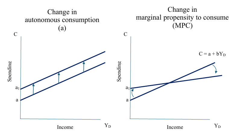
Figure 14 

Let’s examine an economy with autonomous consumption of $100 billion and a 0.50 MPC. This consumption function is depicted in figure 15. For reference, a 45-degree line is presented to show when spending (i.e., consumption) equals income. 

Figure 15 

When income equals $100 billion, spending is about $150 billion. This means that households must either borrow or dip into their savings to cover the $50 billion in spending that exceeds their income. When spending exceeds income, economists refer to this as dissaving. 

On the other hand, when income rises to $400 billion, spending increases to $300 billion. In this case, income exceeds consumption, resulting in savings of $100 billion. 

The only income level where households are not borrowing or saving is when income is $200 billion. At this point, spending exactly equals income, which is represented by the intersection of the consumption function and the 45° line. This is considered a sustainable level of income, because all income is used for consumption without needing to borrow or save.